Regardless how good and flexible the system is, it’s practically impossible to design it in the way that satisfies all customers. Don’t take me wrong – if you have internal development team that works on internal system, you could be fine. But as long as you start to sell the solution or, even better, design the hosting solution for the multiple customers – you are stuck. There is always some customization involved.

One of the very common examples of customization is custom attributes customer wants to store. For example, let’s think about shopping cart system and Article table there. If you put some time trying to define Article attributes you can end up with quite extensive set. Size, Weight, Dimension, Color.. So far so good. But one day sales department close the deal with auto part store and now you have to deal with cylinders, trim types, engine, battery amp-hours and other funny stuff. Next day the company closes the deal with grocery store and you have to deal with nutrition information.

Unfortunately there are no perfect ways to solve the problem. I’m going to show a few obvious and no-so-obvious design patterns that you can use and outline scenarios when those patterns are useful. There will be 3 posts on the suject:

1. Today we will talk about storing attributes in the separate columns and about storing them in XML
2. We will talk about Name/Value table  – there are 2 approaches – very very bad and very very interesting
3. We will do some performance testing and storage analysis for those approaches.

But first, let’s define the set of criteria we are going to use evaluating the patterns:

1. Multiple schema support. Can this solution be used in hosted environments where you have multiple different “custom fields” schema? For example, customer-specific attributes in the system that stores data from the multiple customers (remember auto parts shop and grocery store)
2. Expandability. Does solution offer unlimited expandability in terms of numbers and types of the attributes?
3. Online schema change. E.g. can schema be modified online with active users in the system?
4. Storage cost. How much storage solution requires?
5. Attribute access cost
6. Search-friendliness. How easy is to search for specific value in the attributes scope
7. Sorting/Paging friendliness. How easy is to sort by specific attribute and display specific page based on row number
8. Upfront knowledge of the data schema. What client needs to know about attributes while selecting data.

And before we begin, as the disclaimer. I’m going to show a few patterns but by any means there are other solutions available. Every system is unique and you need to keep your own requirements in mind while choosing the design. Not the best pattern in general could be the best one for specific system and specific requirements.

Pattern 1: One column per attribute

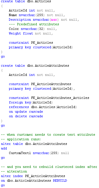
This is probably one of the most common pattern you can find especially in the old systems. There are 3 most common ways how it’s get implemented. In first one, you predefine the set of the custom columns of different types up front and customer is limited by that predefined subset. Something like that (let’s call it 1.a):

Alternatively, there are the systems that dynamically alter the table when customer needs to create the new attribute. Something like that (let’s call it 1.b):

As you can see, I mentioned that rebuilding of clustered index is the good idea. It reduces the index fragmentation due increase of the row size. And if you drop the attribute, you’d need to reclaim the space.

Third variation (let’s call it 1.c) is very similar to 1.b with exception that it stores custom attributes in the separate table:

Let’s evaluate them:

1.  Multiple schema support. It would work with the multiple schema if/when you have predefined set of the attributes (1.a) from above. Of course, in that case all customers will have the limitation on maximum number of attributes per type but it could be acceptable in some systems. In case if you dynamically alter the table only one schema could be supported. Of course, you can do some tricks with that – for example keep multiple tables (one per customer) or reuse the attribute columns created by other customers but either of those approaches would introduce a lot of complexity and management overhead. It’s simply not worth it.
2. Expandability. 1.a obviously is not expandable. At least automatically. 1.b and 1.c offer practically unlimited expandability (subject of SQL Server limitations on max row size and max number of columns).
3. Online schema change. 1.a does not require any physical schema changes. 1.b and 1.c require SCH-M lock acquired on the table during table alteration (which is basically exclusive table access) as well as user should have appropriate rights to execute the ALTER TABLE statement.
4. Storage cost. 1.a – it increases the size of the row in Articles table by the size of all fixed-width data types used by attributes plus at least 2 bytes per variable width attribute regardless if attributes are used or not (see it in more details). This could be OK as long as the table is not transactional (does not store a lot of data) and we are not going crazy with total number of attributes we predefined, but still – it needs to be considered. Row size matters. 1.b and 1.c are much more efficient in that regard – attributes are created only when needed.
5. Attribute access cost. 1.a and 1.b – no overhead at all. Attribute is in the regular column in the row. 1.c – there is the extra join between the tables
6. Search-friendliness. Generally this would introduce the search clause like: where (CustomText1 = @P1) or  (CustomText2 = @P1) ..  Usually those patterns lead to clustered index scans unless there are predicates selective enough to utilize non clustered index. So this is more or less the question if system even need to allow search like that without any additional filters on other columns. One other thing to keep in mind – you need to be careful dealing with various data types and possible conversion errors.
7. Sorting/Paging friendliness. That pattern is extremely friendly for sorting and paging as long as there are some primary filters that limit number of rows to sort/page. Otherwise attribute either needs to be indexed or scan would be involved.
8. Upfront knowledge about the data schema generally is not required. While select * is not the best practice, it would work perfectly when you need to grab entire row with the attributes.

The biggest benefits of that design are simplicity and low access cost. I would consider it for the system that require single data schema (box product) or when multiple data schema would work with limited number of attributes (1.a). While it can cover a lot of systems, in general it’s not flexible enough. I would also be very careful with that pattern in case if we need to add attributes to transactional tables with millions or billions of rows. You don’t want to alter those tables on the fly nor have storage overhead introduced by predefined attributes.

One other possible option is to use SPARSE columns with 1.a and 1.b. SPARSE columns are ordinary columns that optimized for the storage of NULL values. That will technically allow you to predefine bigger set of the attributes than with regular columns without increasing the size of the row. Could be very useful in some cases. Same time you need to keep in mind that not null SPARSE column takes more space than regular column. Another important thing that tables with SPARSE columns cannot be compressed which is another very good way to save on the storage space.

And the last note about the indexing. If you need to support search and/or sort on every attribute you need to either limit the number of rows to process or index every (or most commonly used) attributes. While large number of indexes is not very good thing in general, in some system it’s perfectly OK (especially with filtered indexes that do not index NULL values), as long as you don’t have millions  of rows in the table nor very heavy update activity. Again, this is from “It depends” category.
Pattern 2. Attributes in XML

Well, that’s self-explanatory :). Something like that:

Let’s dive into the details.

1. Multiple schema support. Not a problem at all. You can store whatever you want. As long as it’s the valid XML
2. Expandability. The same. Not a problem at all. Just keep the valid XML and you’re golden
3. Online schema change. Easy. There is no schema on the metadata level. Well, you can, of course, define XML Schema and it will help with performance but again, consider pros and cons of this step.
4. Storage cost. And now we started to talk about negative aspects. It uses good amount of space. XML is basically LOB – SQL Server does not store it in plan text – there are some minor compression involved but still. It uses a lot of space. And if we need to index XML column, it would require even more space
5. Attribute access cost. Heh, and this is another big one. That’s great that SQL Server has build-in XML support. But performance is far from ideal. We will do some performance testing in Part 3 of our discussion but trust me – shredding XML in SQL Server is slow and CPU intensive.
6. Search-friendliness. Well, you need to shred it before the search – it’s very slow. XML Indexes would help but it’s still slower than regular columns and introduce huge storage overhead.
7. Sorting/Paging friendly. Same as above. You need to shred data first.
8. Upfront knowledge about data schema. All data stored in 1 column. So client does not need to jump through any hoops to access the data. But of course, it needs to know how to parse it.

Bottom line – storing custom attributes in XML is the perfect solution in terms of flexibility. Unfortunately it’s very storage-hungry and most importantly very slow in terms of performance. That solution is the best if the main goal is simple attribute storage and displaying/editing very small amount of rows on the client. For example Article detail page on the web site. Although if you need to shred, sort, filter the large number of rows – you’ll have performance issues even with XML Indexes.

Next time we will talk about Name/Value table that deserves the separate post.

I hope everyone had the great holiday season! 🙂

Today I’d like us to talk about Lock Escalation in Microsoft SQL Server. We will cover:

1. What is Lock Escalation?
2. How Lock Escalations affects the system
3. How to detect and troubleshoot Lock Escalations
4. How to disable Lock Escalation

What is Lock Escalation?
All of us know that SQL Server uses row level locking. Let’s think about scenario when system modifies the row. Let’s create the small table and insert 1 row there and next check the locks we have. As usual every image is clickable.

As you can see there are 4 locks in the picture. shared (S) lock on the database – e.g. indication that database is in use. Intent exclusive (IX) lock on the table (OBJECT) – e.g. indication that one of the child objects (row/key in our case) has the exclusive lock. Intent exclusive (IX) lock on the page – e.g. same indication about child object (row/key) exclusive lock. And finally exclusive (X) lock on the key (row) we just inserted.

Now let’s insert another row in the different session (let’s keep the original Session 1 transaction uncommitted).

When we check the locks we will see that there are 8 locks – 4 per session. Both sessions ran just fine and don’t block each other. Everything works smooth – that great for the concurrency. So far so good. The problem though is that every lock takes some memory space – 128 bytes on 64 bit OS and 64 bytes on 32 bit OS). And memory is not the free resource. Let’s take a look at another example. I’m creating the table and populating it with 100,000 rows. Next, I’m disabling the lock escalation on the table (ignore it for now) and clear all system cache (don’t do it in production). Now let’s run the transaction in repeatable read isolation level and initiate the table scan.

Transaction is not committed and as we remember, in repeatable read isolation level SQL Server holds the locks till end of transaction. And now let’s see how many locks we have and how much memory does it use.

As you can see, now we have 102,780 lock structures that takes more than 20MB of RAM. And what if we have a table with billions of rows? This is the case when SQL Server starts to use the process that called “Lock Escalation” – in nutshell, instead of keeping locks on every row SQL Server tries to escalate them to the higher (object) level. Let’s see how it works.

First we need to commit transaction and clear the cache. Next, let’s switch lock escalation for Data table to AUTO level (I’ll explain it in details later) and see what will happen if we re-run the previous example.

As you can see – just 2 locks and only 1Mb of RAM is used (Memory clerk reserves some space). Now let’s look what locks do we have:

As you can see there is the same (S) lock on the database and now we have the new (S) shared lock on the table. No locks on page/row levels are kept. Obviously concurrency is not as good as it used to be. Now, for example, other sessions would not be able to update the data on the table – (S) lock is incompatible with (IX) on the table level. And obviously, if we have lock escalation due data modifications, the table would hold (X) exclusive lock – so other sessions would not be able to read the data either.

The next question is when escalation happens. Based on the documentation, SQL Server tries to escalate locks after it acquires at least 5,000 locks on the object. If escalation failed, it tries again after at least 1,250 new locks. The locks count on index/object level. So if Table has 2 indexes – A and B you have 4,500 locks on the index A and 4,500 locks on the index B, the locks would not be escalated. In real life, your mileage may vary – see example below – 5,999 locks does not trigger the escalation but 6,999 does.

How it affects the system?

Let’s re-iterate our first small example on the bigger scope. Let’s run the first session that updates 1,000 rows and check what locks are held.

As you see, we have intent exclusive (IX) locks on the object (table) and pages as well as various (X) locks on the rows. If we run another session that updates completely different rows everything would be just fine. (IX) locks on table are compatible. (X) locks are not acquired on the same rows.

Now let’s trigger lock escalation updating 11,000 rows.

As you can see – now the table has exclusive lock. So if you run the session 2 query from above again, it would be blocked because (X) lock on the table held by session 1 is incompatible with (IX) lock from the session 2.

When it affects us? There are 2 very specific situations

1. Batch inserts/updates/deletes. You’re trying to import thousands of the rows (even from the stage table). If your import session is lucky enough to escalate the lock, neither of other sessions would be able to access the table till transaction is committed.
2. Reporting – if you’re using repeatable read or serializable isolation levels in order to have data consistent in reports, you can have (S) lock escalated to the table level and as result, writers will be blocked until the end of transaction.

And of course, any excessive locking in the system can trigger it too.

How to detect and troubleshoot Lock Escalations

First of all, even if you have the lock escalations it does not mean that it’s bad. After all, this is expected behavior of SQL Server. The problem with the lock escalations though is that usually customers are complaining that some queries are running slow. In that particular case waits due lock escalations from other processes could be the issue. If we look at the example above when session 2 is blocked, and run the script (as the session 3) that analyzes sys.dm_tran_locks DMV, we’d see that:

I’m very heavy on the wait statistics as the first troubleshooting tool (perhaps heavier than I need to be 🙂 ). One of the signs of the issues with lock escalations would be the high percent of intent lock waits (LCK_M_I*) together with relatively small percent of regular non-intent lock waits. See the example below:

In case if the system has high percent of both intent and regular lock waits, I’d focus on the regular locks first (mainly check if queries are optimized). There is the good chance that intent locks are not related with lock escalations.

In addition to DMVs (sys.dm_tran_locks, sys.dm_os_waiting_tasks, sys.dm_os_wait_stats, etc), there are Lock Escalation Profiler event and Lock Escalation extended event you can capture. You can also monitor performance counters related with locking and create the baseline (always the great idea)

Last but not least, look at the queries. As I mentioned before in most part of the cases excessive locking happen because of non-optimized queries. And that, of course, can also trigger the lock escalations.

How to disable Lock Escalation

Yes, you can disable Lock Escalations. But it should be the last resort. Before you implement that, please consider other approaches

1. For data consistency for reporting (repeatable read/serializable isolation levels) – switch to optimistic (read committed snapshot, snapshot) isolation levels
2. For batch operations consider to either change batch size to be below 5,000 rows threshold or, if it’s impossible, you can play with lock compatibility. For example have another session that aquires IS lock on the table while importing data. Or use partition switch from the staging table if it’s possible

In case if neither option works for you please test the system before you disable the lock escalations. So:

For both SQL Server 2005 and 2008 you can alter the behavior on the instance level with Trace Flags 1211 and 1224. Trace flag 1211 disables the lock escalation in every cases. In case, if there are no available memory for the locks, the error 1204 (Unable to allocate lock resource) would be generated. Trace flag 1224 would disable lock escalations in case if there is no memory pressure in the system. Although locks would be escalated in case of the memory pressure.

With SQL Server 2005 trace flags are the only options you have. With SQL Server 2008 you can also specify escalation rules on the table level with ALTER TABLE SET LOCK_ESCALATION statement. There are 3 available modes:

1. DISABLE – lock escalation on specific table is disabled
2. TABLE (default) – default behavior of lock escalation – locks are escalated to the table level.
3. AUTO – if table is partitioned, locks would be escalated to partition level when table is partitioned or on table level if table is not partitioned

Source code is available for download

Part 13 – Schema locks

Table of content

Long time ago we discussed that good clustered index needs to be unique, static and narrow. I mentioned that internally SQL Server needs to be able to unique identify every row in the table (think about non-clustered index key lookup operation) and in case, if clustered index is not defined as unique, SQL Server adds 4 bytes uniquifier to the row. Today I want us to talk about that case in much more details and see when and how SQL Server maintains that uniquifier and what overhead it introduces.

In order to understand what happens behind the scene we need to look at the physical row structure and data on the page. First, I have to admit, that general comment about 4 bytes uniquifier overhead was not exactly correct. In some cases overhead could be 0 bytes but in most cases it would be 2, 6 or 8 bytes. Let’s look at that in more details. Click on the images below to open them in the new window.

First, let’s create 3 different tables. Each of them will have only fixed-width columns 1000 bytes per row + overhead. So it gives us an ability to put

• UniqueCI – that table has unique clustered index on KeyValue column
• NonUniqueCINoDups – that table has non unique clustered index on KeyValue column. Although we don’t put any KeyValue duplicates to that table
• NonUniqueCIDups – that table has non unique clustered index on KeyValue column and will have a lot of duplicates.

Now let’s add some data to those tables.

First, let’s take a look at the physical stats on the clustered index. Two things are interesting. First – Min/Max/Avg record size, and second is the Page Count.

As you can see, best case scenario in UniqueCI table has 1007 bytes as Min/Max/Avg record size (again – all columns are fixed width) and uses 12500 pages. Each page can store 4 rows (1,007 bytes per row * 8 = 8,056 bytes < 8,060 bytes available on the page.

Next, let’s take a look at NonUniqueCINoDups table. Even if clustered index is not unique, Min/Max/Avg/Page Count are the same with UniqueCI clustered index. So as you can see, in this particular case of non-unique clustered index, SQL Server keeps null value for uniquifier for the first (unique) value of the clustered index. And we will look at it in more details later.

The last one – NonUniqueDups table, is more interesting. As you can see, if Min record size is the same (1,007 bytes), Maximum is 1,015 bytes. And Average record size is 1,014.991 – very similar to the maximum record size. Basically, uniquifier value added to all rows with exception of the first row per unique value. Interestingly enough that even if uniquifier itself is 4 bytes the total overhead is 8 bytes.

Another thing is worth to mention is the page count. As you can see, there are 1,786 extra pages (about extra 14M of the storage space). 8 rows don’t fit on the page anymore. Obviously this example does not represent real-life scenario (no variable with columns that can go off-row, etc) although if you think about non-clustered indexes, the situation is very close to the real-life. Let’s create non-clustered indexes and checks the stats.

As you can see, in the latter case, we almost doubled the size of the non-clustered index leaf row and storage space for the index. That makes non-clustered index much less efficient.

Now let’s take a look at the actual row data to see how SQL Server stores uniquifier. We will need to take a look at the actual data on the page. So the first step is to find out what is the page number. We can use DBCC IND command below. Let’s find the first page on the leaf level (the one that stores very first row from the table). Looking at DBCC IND result set, we need to select PagePID for the IndexLevel = 0 and PrevPageFID = 0.

Next, we need to run DBCC PAGE command and provide that PagePID. Both DBCC IND and DBCC PAGE are perfectly save to run on the production system. One other thing you need to do is to enable trace flag 3604 to allow DBCC PAGE to display result in the console rather than put it to SQL Server error log.

So let’s take a look at the row itself. First, we need to remember that DBCC PAGE presents multi-byte values with least-significant bytes first (for example int (4 bytes) value 0x00000001 would be presented as 0x01000000). Let’s take a look at the actual bytes.

• Byte 0 (TagByteA) (green underline) – this is the bit mask and in our case 0x10 means that there is NULL bitmap
• Byte 1 (TagByteB) – not important in our case
• Byte 2 and 3 (yellow underline) – Fixed width data size
• Bytes 4+ stores the actual fixed width data. You can see values 0x01 (0x10000000 in reverse order) for KeyValue and ID and ‘a..’ for the CharData columns.

But much more interesting is what we have after Fixed-Width data block. Let’s take a look:

Here we have:

• Number of columns – 2 bytes (Red underline): 0x0300 in reverse order – 3 columns that we have in the table.
•  Null bitmap (Blue underline): 1 byte in our case – no nullable columns – 0.

So everything is simple and straightforward. Now let’s take a look at NonUniqueCINoDups data. Again, first we need to find the page id with DBCC IND and next – call DBCC PAGE.

I’m omitting first part of the row – it would be exactly the same with UniqueCI row. Let’s take a look at the data after fixed-width block.

As you can see, number of columns (Red underline) is now 4 that includes uniquifier which does not take any physical space. And if you thinking about it for a minute – yes, uniquifier is nullable int column that stores in the variable-width section of the row. SQL Server omits data for nullable variable width columns that are the last in the variable-width section which is the case here. If we had any other variable width columns with the data, uniquifier would use two bytes in the offset array even if value itself would be null.

And now let’s take a look at NonUniqueCIDups rows. Again, DBCC IND, DBCC PAGE.

If we look at the variable width section of the first row in the duplication sequence), it would be exactly the same with NonUniqueCINoDups. E.g. uniquefier does not take any space.

But let’s look at the second row.

Again we have:

• Number of columns – 2 bytes (Red underline): 4
• Null bitmap (Blue underline)
• Number of variable-width columns – 2 bytes (Green underline) – 0x0100 in reverse order – 1 variable width column
• Offset of variable-width column 1 – 2 bytes (Black underline)
• Uniquefier value – 4 bytes (purple underline)

As you can see, it introduces 8 bytes overhead total.

To summarize storage-wise – if clustered index is not unique then for unique values of the clustered key:

• There is no overhead if row don’t have variable-width columns or all variable-width columns are null
• There are 2 bytes overhead (variable-offset array) if there is at least 1 variable-width column that stores not null value

For non-unique values of the clustered key:

• There are 8 extra bytes if row does not have variable-width columns
• There are 6 extra bytes if row has variable-width columns

This applies not only to the clustered indexes but also to non-clustered index that references clustered index key values. Well, storage is cheap but IO is not..

Source code is available for download

P.S. Happy Thanksgiving! 🙂

We all already know that in most part of the cases deadlocks happen due non-optimized queries. Today I’d like to show another pattern that could lead to the deadlocks. It’s not something that happens very often but it’s worth to mention.

Let’s think about the following scenario. Assuming you have the system that collects some data from the users. Assuming the data has a few parts that can be processed and saved independently from each other. Also let’s assume that there is some processing involved – let’s say there is a raw data part and something system needs to calculate based on that.

One of the approaches to architect the system is separating those updates and processing to the different threads/sessions. It could make sense in some cases – data is independent, threads and sessions would update different columns so even if they start updating the row simultaneously, in the worst case one session would be blocked for some time. Nothing terribly wrong as long as there are no multiple updates of the same row involved. Let’s take a look.

First, let’s create the table and populate it with some data:

Now let’s run the first session, open transaction and do the update of RawData1 column. Also, let’s check the plan. This update statement used non-clustered index seek/key lookup – keep this in mind, it would be important later.

Now let’s run the second session that updates different column on the same row. Obviously this session is blocked – first session holds (X) lock on the row.

Now let’s come back to the first session and try to update another column on the same row. This is the same session that holds (X) row so it should not be the problem.

But.. We have the deadlock.

Why? Let’s take a look at deadlock graph (click to open the new window)

So on the right we have the first session. This session holds the (X) lock on the clustered index row (PK_Users). When we ran the session 2 statement, that session obtained (U) lock on non-clustered index row (IDX_Users_ExternalID), requested (U) lock on the clustered index and was blocked because of the first session (X) lock. Now, when we ran the second update statement from the first session, it tries to request the (U) lock on the non-clustered index and obviously was blocked because the second session still holds (U) lock there. Classic deadlock.

As you can see, it happened because SQL Server uses non-clustered index seek/key lookup as the plan. Without non-clustered index seek everything would work just fine.

This is quite interesting scenario and you can argue that it does not happen often in the real life. Well, yes and no. If we think about 2 update statements in the row – yes – usually we don’t write code that way. But think about stored procedures. If the processing can be done/called from a few different places, you can decide to put the update to the stored procedure. And here you go.

But most importantly – there are the triggers. What if you have AFTER UPDATE trigger and want to update some columns from there. Something like that:

Now let’s run update statement in the first session.

And in the second session.

Deadlock again. You can notice that I used ExternalId and as result non-clustered index seek/key lookup plan there. It does not make a lot of sense in this scenario – I could use UserId there and avoid the problem. So if you have to update original row from the trigger – be careful and write the query in the way that introduces clustered index seek.

Source code is available for download

Part 12 – Lock Escalation

Table of content

Wrapping up.. Only remaining question is “What isolation level is good for me”? And there is no right answer to that question. As usual, it depends. I’ll try to summarize a few things but again, think about specific details of your system and make decision based on them, not on generic advices below.

When you start to think what isolation level should you use in your system, there are 2 questions you need to answer. First, what is the blueprint of your system – is it OLTP or Data Warehouse type system? OLTP systems usually handles operational activity of the company and serves high volume of short identical queries and short transactions. Data Warehouse blueprint described reporting type system with low volume of long transactions and complex queries. In OLTP systems data is constantly changing, in Data Warehouse systems it rarely the case – data usually updates on the batches based on some schedule.

As the example, let’s think about online store. The database that handles customer facing shopping cart web site is OLTP. There are always new orders coming, existing order updating, customers check the status of existing orders, search the article lists, etc – those are done within short transactions and simple queries. Assuming same time company executives want to run some reports, see some trends and other analysis – there is the good chance that it would be another database for that purpose. This database would be optimized for complex reporting and data in that database could be refreshed every night or perhaps on the weekly basis. That database is Data Warehouse.

In real life, of course, it’s rarely the case. There is always some reporting activity against OLTP database but in any case, you can see what blueprint fits better. And it leads to the second question you need to answer: “How much data consistency do I really need?”. And even if the answer “I don’t need any consistency” is quite popular, it rarely the case in the real life. So let’s dive a little bit more in “no-consistency” mode.

No-consistency in terms of transaction isolation levels mean read uncommitted. Either directly as “set transaction isolation level” or with (NOLOCK) hints. There are some cases when you can decide to use that isolation level – for example, in our system we have a few transaction entities where data has been inserting to our system and never ever updating/deleting after that. Same time, clients are constantly downloading the data and we don’t really care if clients get the data from uncommitted transaction. This is the case when we can downgrade to read uncommitted isolation level to reduce the blocking for the client downloading sessions.

But if you think about that example – it’s rather exception than the rule. In most part of the systems you want to have consistency. Think about reporting for executives – how happy they would be if you provided them incorrect data or, even better, if they get different results running the same report twice? And the real problem that in the real life people often switches to read uncommitted isolation level to solve the blocking issues. Right, it could help in the cases when select queries (readers) are blocked by update queries (writers). But it’s rather masking the problem than solving it. As we already know, in most part of the cases, locking and blocking issues triggered by non-optimized queries. So, if you had a chance, you’d better spend some time on query optimization. Of course, this advice would not help if you are in fire-drill mode and need to fix the blocking issues in production system but in such case there is another option that could work even better – use read committed snapshot instead of
read uncommitted. In that mode writers also don’t block readers and same time give you statement level consistency. Of course there are some performance implications but in most part of the cases you can live with them.

Read committed, which is also default isolation level, in most part of the cases (again, assuming the system is more or less optimized) – this is the good choice especially for OLTP systems. It gives you acceptable compromise between consistency and concurrency. Again, there is blocking involved but when system is optimized – it’s minimal. Speaking of higher isolation levels – repeatable reads and serializable – those are typically bad choice for OLTP. For reporting and data warehouse systems those could be acceptable but same time for such systems optimistic isolation levels (read committed snapshot and snapshot) are better.

And speaking of optimistic isolation levels. For Data Warehouse type systems – use them. I don’t think about any single reason why you would like to avoid them in such systems. For OLTP – consider them. If you can live with performance overhead – it could be the good choice. Be careful – don’t forget about extra 14 bytes and don’t use fillfactor = 100 though.

So, the bottom line. For Data Warehouse – use optimistic isolation levels whenever possible. Only case with Data Warehouse systems when I would suggest to consider different options is when data in the system updates on the real time. And even in such case give optimistic isolation levels the try. For OLTP – if you can use optimistic isolation levels – use them (start with read committed snapshot). If not, use read committed and optimize the queries. Don’t use read uncommitted and (nolock) hints unless you don’t care at all about consistency. And definitely don’t use read uncommitted to reduce blocking. This is the bad choice.

Last, but not least, don’t forget that you can, and often need to use multiple different isolation levels in the system. Use them wisely! 🙂

Part 11 – Deadlocks due multiple updates of the same row

Table of content

Two week ago we discussed 2 “optimistic” transaction isolation levels – Snapshot and Read Committed Snapshot. We already saw how those isolation levels can provide us transaction and statement level consistency reducing blocking issues same time. Sounds too good to be true..

So does it make sense to switch to optimistic isolation levels? Well, the answer is typical – “it depends”. There are a few things you need to keep in mind before you make the decision. Let’s talk about them from both – DBA and Database Developer standpoints.

First of all, as we already know, optimistic isolation levels use tempdb for the version store. When you modified the row, one or more old versions of the row is stored in tempdb. This leads to the higher tempdb load as well as to the larger tempdb size. Would it be the issue for your system? Again, it depends. As the bare minimum you should reserve enough space for tempdb and closely monitor the load. There are a few performance counters under <SqlInstance>:Transactions section that related to the version store – they will show you version store size, generation and cleanup rates and a few other parameters. Those are very useful and I recommend to add them to your baseline.

Second thing you need to keep in mind is that SQL Server needs to store additional 14 bytes pointer to the version store in the. It’s not only increasing the row size, it also can introduce page splits. Let’s take a look. Let’s use the same database from the last blog post – you can download it from the last post.

Let’s rebuild the index (with default FILLFACTOR=100) and look at the index statistics (click on the image to open it in the different window). As you can see, it has 0% fragmentation. Row size is 215 bytes.

Now let’s run transaction in snapshot isolation level and update Value column. This is integer (fixed width column) so this update by itself should not increase row size. If you look at the index statistics now, you can see that there were heavy page splits and row size increased by 14 bytes. Those 14 bytes is the pointer to the version store.

The bottom line – if you use optimistic isolation level, don’t use 100% fillfactor for the indexes.

Speaking of development challenges – well, it’s become a little bit more interesting. First potential program is referential integrity based on triggers. Let’s take a look. Let’s create 2 tables – MasterData and DetailData and after insert trigger on DetailData. In this trigger let’s check that master data exists and rollback transaction in case of referential integrity violation. Let’s test that:

Now let’s move to more complex scenario and 2 sessions. First, let’s start transaction in the 1st session and check if we have MasterData row.

Let’s keep transaction open and in the second session let’s delete master data row. As you see everything is just fine.

Next, lets come back to the first session and insert detail row that references the master row – as you can see there is no errors but referential integrity has been compromised.

It happens because inside the trigger we still are in the context of the old transaction where we reference old version of MasterData row from the version store. This could be easily fixed in the trigger by using (READCOMMITTED) query hint but of course you should remember it and modify the code. It worth to mention that regular referential integrity based on foreign keys uses read committed isolation level by default.

Another issue is the update of the same row. Let’s take a look. first let’s reset Master and Detail table data. Now let’s start transaction in the first session and query the data

Next, let’s update data row in another transaction from another session

And now let’s try to update the same row from the first session and commit the transaction.

As you can see, behavior is completely different from the regular pessimistic isolation levels – it raises the exception. So obviously the client application needs to catch those errors and either notify users or implement some sort of retry logic to handle it.

And finally let’s look at the different update behavior in snapshot isolation mode. Let’s start the transaction assuming we have 2 rows in the table

Next, in another session let’s run update that changes DetailDataId to 2 for the first row.

Now in the first session let’s do the opposite action and check results

As you see, because of the row versioning it simply swaps the values. It would be completely different with regular pessimistic isolation levels when one session would be blocked and next update either 0 or 2 rows (depend on what session acquires the lock first). The bottom line – if you move your application to snapshot isolation level, you need to test how it would behave in environment with the multiple users. Otherwise you’d have a few nice side effects.

So to summarize – optimistic isolation levels are great but you have to keep a few things in mind:

• Extra tempdb load
• Possible page splits/fragmentations due bigger row size
• Referential integrity based on triggers does not work unless read committed hint is used
• There are different behaviors for updates when multiple sessions update the same rows and when scan is involved.

Source Code is available for download

Part 10 – What isolation level should I choose?

Table of content

There was some time since we discussed locking and blocking in Microsoft SQL Server. One big area we did not cover is optimistic transaction isolation levels. So what exactly are those?

As you remember, standard “pessimistic” isolation levels – read uncommitted, read committed and repeatable read – all of them can have anomalies. Dirty and non-repeatable reads, ghost rows and duplicated reads. Higher isolation levels reduce anomalies in price of reduced concurrency. Most restrictive – Serializable isolation level guarantees no anomalies although with such level concurrency greatly suffers. Before SQL Server 2005 it was virtually impossible to have consistent reporting in the systems with heavy reading and writing activities.

Obviously in quite competitive market Microsoft had to do something to solve that problem. As the result, one of the features Microsoft introduced in SQL Server 2005 was new “optimistic” transaction isolation levels. With those isolation levels readers use row versions rather than locking. When you start the transaction and modify some rows, old version of the rows are copied to the version store in tempdb. Actual row holds 14 bytes pointer to the version store.

There are 2 different isolation levels – well, actually one and half. First one is called Read Committed Snapshot and not really the level but more or less the mode of Read Committed. This level implements statement level consistency – readers would not be blocked by writers but in transaction scope it could have same anomalies as regular read committed (with the exception of duplicated reads). Let’s take a look. If you don’t have test database, create it first. First, let’s enable read committed snapshot isolation level. It worth to mention that when you switch the mode, you should not have any users connected to the database.

Next, let’s create the table and populate it with some data

Now let’s start one session and update one of the rows. As you can see, this session starts in read committed isolation level

Let’s look at the locks we have in the system. As you can see, we have exclusive lock on the row. This is expected and should happen with any isolation level. Click to the image to open it in the different window

Now let’s start another session and try to select the same row.

And here is the big difference with regular read committed. Instead of being blocked as when we have pessimistic isolation level, it returns old version of the row with placeholder equal ‘a’. So far, so good. Now let’s run another update.

As you can see, with read committed snapshot we still have writers acquiring U and X locks – so those statements would be blocked as with regular pessimistic isolation levels. What does it really mean for us? If your system suffers because of the blocking between readers and writers, read committed snapshot helps in such situation – blocking would be reduced. This is especially good if you need to deal with 3rd party vendors databases – you can change the database option and (partially) solve the problem. Although read committed snapshot would not help if writers block each other. you’ll still have typical update and exclusive locks behavior.

One other thing I already mentioned – read committed snapshot does not provide you consistency on the transaction scope. Consistency is guaranteed only on the statement scope. Let’s check that:

Now let’s commit the session 1 (I don’t put screen shot here) and run select statement again. We’re on the same transaction context.

As you can see, select returns new (updated) row value. Again, no transaction level consistency in such case. If you need full consistency on transaction level, you need to use SNAPSHOT isolation level. With such isolation level SQL Server stores multiple “old” versions of the row – as long as there are transactions that can reference them. When session references the row, it reads the version that was valid on the moment when transaction started. It has “snapshot” of the data for the transaction.

Let’s take a look. First, you need to enable that option on database level. Again, you need to be on single user mode in order to do so.

Next, let’s run same update statement and keep transaction uncommitted.

Now let’s go to another session, start transaction in snapshot isolation level and see what happens.

First, let’s select of the row updated by another session that holds X lock. As you can see – same behavior with read committed snapshot – it returns old value.

Now let’s try to update another row with table scan. As you can see – no blocking due U/X lock incompatibility now. Both rows have been updated, 2 X locks held

Now let’s commit transaction in the first session and run select in the second session again. It still returns the data that you had at the time when transaction was just started. Even if that row has been modified.

And now let’s delete that row in the first session.

If you run same select in the second session – it still returns that row.

As you can see, this is consistency on the transaction level. SQL Server guarantees that data within the transaction would be exactly the same during transaction lifetime. Even if it looks similar to Serializable isolation level, there is the key difference. With Serializable level you “lock” the data on the moment you access it. With Snapshot, it “locked” on the moment when transaction started. And obviously, this is the Heaven for reporting – consistent data with no blocking.

Too good to be true. Yes, there are a few things you need to keep in mind from both DBA and Development prospective. And we will talk about them next time.

Source code is available for download

Part 9 – Optimistic transaction isolation levels – TANSTAAFL! 

Also take a look at Part 15 – When Transaction Starts. It gives some additional details about snapshot isolation level

Table of content