Category Archives: T-SQL

Blocking Monitoring Framework: Capture and Analyze SQL Server Blocking and Deadlock Information With Event Notifications

If you worked with SQL Server for a while, you should have noticed how landscape changed over the years. We are dealing with the different problems now. Five years ago, majority of the issues I saw were related to non-optimized queries. There were the huge scans with a lot of  physical I/O and bad performance.

You do not see them as often nowadays. It is very cheap to solve the problems by upgrading the server. Put a couple hundred GBs of RAM and cache all the data; add more CPUs and problems magically disappear. The root-cause has not been fixed but who cares?

Surprisingly, there is one category of the issues that did not went away – concurrency. It even becomes worse. Modern servers handle more users and problems that did not exist with 50 concurrent users may put the server to its knees with 5000 users. I’ve been constantly involved in the troubleshooting of various concurrency issues and, in fact, I see more and more of them overtime.

Troubleshooting of the blocking and concurrency issues is, in the nutshells, a simple process. You need to identify the processes involved in blocking conditions or deadlocks and analyze why those processes acquire the locks on the same resources. In majority of cases, you need to analyze queries and their execution plans identifying possible inefficiencies that led to excessive number of locks being acquired.

Collecting this information is not a trivial task. The information is exposed through DMVs (you can download the set of scripts here); however, it requires you to run the queries at time when blocking occurred. Fortunately, SQL Server allows you to capture blocking and deadlock conditions with the blocked process report and deadlock graph, analyzing them later.

There is the caveat though. Neither blocked process report nor deadlock graph provide you execution plans of the statements. Nor do they always include affected statements in the plain text. You may need to query plan cache and other DMVs to get this information and longer you wait lesser is the chance that the information is available. Moreover, SQL Server may generate enormous number of blocked process reports in cases of prolonged blocking and complex blocking chains, which complicates the analysis.

This analysis may become very time consuming, especially if you need to deal with the large number of servers. Over the years, I have created the set of routines, which simplify it for me. I have been thinking to publish my scripts for a while, but I’ve never had time to polish them enough for public consumption. Until now – and I am very happy to share my collection with all of you. So allow me introduce the Blocking Monitoring Framework, which I am using with majority of my servers!

This framework is using Event Notifications. It captures blocked process report and deadlock graphs and parses them at time when event occurred and all data is still available in the system. All information is persisted in the set of tables for the further analysis.

The first version is available for download. I also promise you that I am going to support and enhance it in the future publishing the new versions on the regular basis.

Please feel free to contact me in case of any questions. I would also appreciate if you provide me any blocked process reports and deadlock graphs that framework was unable to parse. I will address the issues as quickly as I could.

Blocking Monitoring Framework

Locking in Microsoft SQL Server (Part 21) – Intro Into Transaction Management and Error Handling

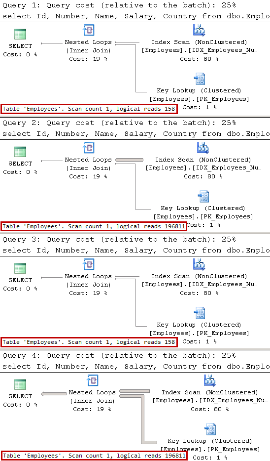
As strange as it sounds, I have never considered transaction management to be the topic that requires explanation. However, it seems that some aspects of it are confusing and may benefit from the separate, long overdue, blog post.

Transaction Types

There are three types of transactions in SQL Server – explicit, autocommitted and implicit.

Explicit transactions are explicitly controlled by the code. You can start them by using BEGIN TRAN statement. They will remain active until you explicitly call COMMIT or ROLLBACK in the code.

In case, when there are no active transactions present, SQL Server would use autocommitted transactions – starting transactions and committing them for each statement it executes. Autocommitted transactions work on per-statement rather than per-module level. For example, when a stored procedure consists of five statements; SQL Server would have five autocommitted transactions executed. Moreover, if this procedure failed in the middle of execution, SQL Server would not roll back previously committed autocommitted transactions. This behavior may lead to logical data inconsistency in the system.

For the logic that includes multiple data modification statements, autocommitted transactions are less efficient than explicit transactions due to the logging overhead they introduce. In this mode, every statement would generate transaction log records for implicit BEGIN TRAN and COMMIT operations, which leads to the large amount of transaction log activity and degrade performance of the system.

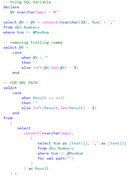
There is another potential performance hit caused by excessive number of autocommitted transactions. As you know, SQL Server implements Write-Ahead Logging to support transaction durability hardening log records on-disk synchronously with data modifications. Internally, however, SQL Server batches log write operations and caches log records in memory in small 60KB structures called log buffers. COMMIT log record forces SQL Server to flush log buffers to disk introducing synchronous I/O operation.

Figure 1 illustrates this condition. INSERT_1, UPDATE_1 and DELETE_1 operations run in autocommitted transactions generating additional log records and forcing log buffer to flush on each COMMIT. Alternatively, INSERT_2, UPDATE_2 and DELETE_2 operations run in implicit transaction, which leads to more efficient logging.

01. Transaction Logging with Autocommitted and Explicit Transactions

You can run the code below to see this overhead in action. It performs INSERT/UPDATE/DELETE sequence 10,000 times in the loop in autocommitted and explicit transactions respectively, measuring execution time and transaction log throughput with sys.dm_io_virtual_file_stats view.

create table dbo.TranOverhead
(
    Id int not null,
    Col char(50) null,
    constraint PK_TranOverhead
    primary key clustered(Id)
);

-- Autocommitted transactions
declare
    @Id int = 1,
    @StartTime datetime = getDate(),
    @num_of_writes bigint,
    @num_of_bytes_written bigint

select @num_of_writes = num_of_writes, @num_of_bytes_written = num_of_bytes_written
from sys.dm_io_virtual_file_stats(db_id(),2);

while @Id < 10000
begin
    insert into dbo.TranOverhead(Id, Col) values(@Id, 'A');

    update dbo.TranOverhead set Col = 'B' where Id = @Id;

    delete from dbo.TranOverhead where Id = @Id;

    set @Id += 1;
end;

select 
    datediff(millisecond, @StartTime, getDate()) as [Exec Time ms: Autocommitted Tran]
    ,s.num_of_writes - @num_of_writes as [Number of writes]
    ,(s.num_of_bytes_written - @num_of_bytes_written) / 1024 as [Bytes written (KB)]
from
    sys.dm_io_virtual_file_stats(db_id(),2) s;
go

-- Explicit Tran
declare
    @Id int = 1,
    @StartTime datetime = getDate(),
    @num_of_writes bigint,
    @num_of_bytes_written bigint

select @num_of_writes = num_of_writes, @num_of_bytes_written = num_of_bytes_written
from sys.dm_io_virtual_file_stats(db_id(),2);

while @Id < 10000
begin
    begin tran
        insert into dbo.TranOverhead(Id, Col) values(@Id, 'A');

        update dbo.TranOverhead set Col = 'B' where Id = @Id;

        delete from dbo.TranOverhead where Id = @Id;
    commit
    set @Id += 1;
end;

select 
    datediff(millisecond, @StartTime, getDate()) as [Exec Time ms: Explicit Tran]
    ,s.num_of_writes - @num_of_writes as [Number of writes]
    ,(s.num_of_bytes_written - @num_of_bytes_written) / 1024 as [Bytes written (KB)]
from
    sys.dm_io_virtual_file_stats(db_id(),2) s;

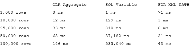
In my environment and this test, explicit transactions are about two times faster and generated three less log activity than autocommitted ones as shown in Figure 2.

02. Explicit and Autocommitted Transaction Performance

As the side note, SQL Server 2014 and above allows you to improve transaction log throughput by using delayed durability. In this mode, SQL Server does not flush log buffers when COMMIT log records are generated. This reduces the number of disk writes at cost of potential small data loss in case of disaster.

SQL Server also supports implicit transactions, which you can enable with SET IMPLICIT_TRANSACTION ON statement. When this option is enabled, SQL Server starts the new transaction when there is no active explicit transactions present. This transaction stays active until you explicitly issue COMMIT or ROLLBACK statement.

Implicit transactions may make transaction management more complicated and they are rarely used in production. However, there is the caveat – SET ANSI_DEFAULT ON option also automatically enables implicit transactions. This behavior may lead to unexpected concurrency issues in the system.

Error Handling

The error handling in SQL Server is the tricky subject especially with transactions involved. SQL Server would handle exceptions differently depending on error severity, active transaction context and several other factors.

Let’s look how exceptions affect control flow during execution. Listing below creates two tables- dbo.Customers and dbo.Orders – and populates them with the data. Note the existence of foreign key constraint defined in dbo.Orders table.

create table dbo.Customers
(
    CustomerId int not null,
    constraint PK_Customers
    primary key(CustomerId)
);

create table dbo.Orders
(
    OrderId int not null,
    CustomerId int not null,

    constraint FK_Orders_Customerss
    foreign key(CustomerId)
    references dbo.Customers(CustomerId)
);
go

create proc dbo.ResetData
as
begin
    begin tran
        delete from dbo.Orders;
        delete from dbo.Customers;
        insert into dbo.Customers(CustomerId) values(1),(2),(3);
        insert into dbo.Orders(OrderId, CustomerId) values(2,2);
    commit
end;

exec dbo.ResetData;

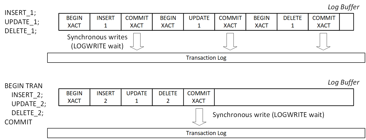
Let’s run three DELETE statements in one batch as shown below. The second statement will trigger a foreign key violation error. @@ERROR system variable provides the error number for the last T-SQL statement executed (0 means no errors).

delete from  dbo.Customers where CustomerId = 1; -- Success
select @@ERROR as [@@ERROR: CustomerId = 1];
delete from  dbo.Customers where CustomerId = 2; -- FK Violation
select @@ERROR as [@@ERROR: CustomerId = 2];
delete from  dbo.Customers where CustomerId = 3; -- Success
select @@ERROR as [@@ERROR: CustomerId = 3];
go

select * from dbo.Customers;

Figure 3 illustrates the output of the code. As you can see, SQL Server continues execution after non-critical foreign key violation error deleting a row with CustomerId=3 afterwards.

03. Running Three Autocommitted Transactions in a Batch

The situation would change when you use TRY..CATCH block as shown below.

exec dbo.ResetData;
go

begin try
    delete from  dbo.Customers where CustomerId = 1; -- Success
    delete from  dbo.Customers where CustomerId = 2; -- FK Violation
    delete from  dbo.Customers where CustomerId = 3; -- Not executed
end try
begin catch
    select 
        ERROR_NUMBER() as [Error Number]
        ,ERROR_LINE() as [Error Line]
        ,ERROR_MESSAGE() as [Error Message];
end catch
go

select * from dbo.Customers;

As you can see in Figure 4, the error was caught in the CATCH block and the third deletion statement has not been executed.

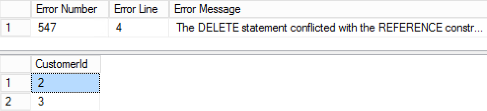
04. Running Three Autocommitted Transactions in TRY..CATCH block

Remember that non-critical exceptions do not automatically rollback explicit or implicit transactions regardless if TRY..CATCH block is present. You still need to commit or rollback transaction after the error.

Depending on severity of the error, transaction in which error occurred may be committable or become uncommittable and doomed. SQL Server would not allow you to commit uncommittable transactions and you must roll it back to complete it.

The XACT_STATE() function allows you to analyze the state of transaction and it returns one of three values:

  • 0 indicates that there is no active transactions present.
  • 1 indicates that there is an active and committable transaction present. You can perform any actions and data modifications committing transactions afterwards.
  • -1 indicates that there is an active uncommittable transaction present. You cannot commit such transaction.

There is very important SET option- XACT_ABORT– which allows you to control error-handling behavior in the code. When this option is set to ON, SQL Server treats every run-time error as severe, making transaction uncommittable. This prevents you from accidentally committing transactions when some data modifications failed with non-critical errors.

When XACT_ABORT is enabled, any error would terminate the batch when TRY..CATCH block is not present. For example, if you run the code from the second code sample above again using SET XACT_ABORT ON, the third DELETE statement would not be executed and only the row with CustomerId=1 will be deleted. Moreover, SQL Server would automatically rollback doomed uncommitted transaction after the batch completes.

The code below shows this behavior. The stored procedure dbo.GenerateError sets XACT_ABORT to ON and generates an error within the active transaction. @@TRANCOUNT variable returns the nested level of transaction (more on it later) and non-zero value indicate that transaction is active.

create proc dbo.GenerateError
as
begin
    set xact_abort on
    begin tran
        delete from dbo.Customers where CustomerId = 2; -- Error
        select 'This statement will never be executed';
end
go

exec dbo.GenerateError;
select 'This statement will never be executed';
go

-- Another batch
select XACT_STATE() as [XACT_STATE()], @@TRANCOUNT as [@@TRANCOUNT];
go

Figure 5 illustrates the output of the code. As you can see, batch execution has been terminated and transaction has been automatically rolled back at the end of the batch.

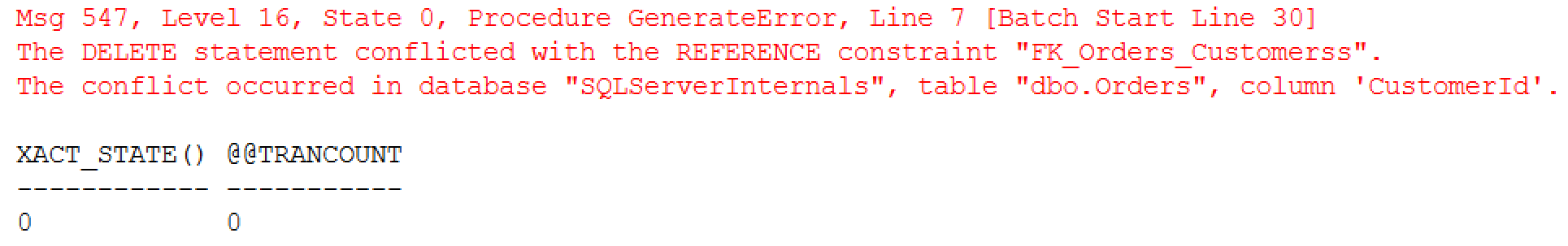
505. XACT_ABORT behavior (no TRY..CATCH block)

TRY..CATCH block, however, will allow you to capture the error even with XACT_ABORT set to ON.

begin try
    exec dbo.GenerateError;
    select 'This statement will never be executed';
end try
begin catch
    select 
        ERROR_NUMBER() as [Error Number]
        ,ERROR_PROCEDURE() as [Procedure]
        ,ERROR_LINE() as [Error Line]
        ,ERROR_MESSAGE() as [Error Message];

    select 
        XACT_STATE() as [XACT_STATE()]
        ,@@TRANCOUNT as [@@TRANCOUNT];

    if @@TRANCOUNT > 0
        rollback;
end catch

As you can see in Figure 6, exception has been trapped in the CATCH block with transaction still remain active there.

06. XACT_ABORT Behavior (with TRY..CATCH block)

Consistent error handling and transaction management strategies are extremely important and allow to avoid data consistency errors and improve data quality in the system. I would recommend the following approach as the best practice:

  • Always use explicit transactions in the code during data modifications. This would guarantee data consistency in transactions that consists of multiple operations. It is also more efficient comparing to individual autocommitted transactions.
  • Set XACT_ABORT to ON before data modifications. This would guarantee “all-or-nothing” behavior of the transaction preventing SQL Server from ignoring non-severe errors and committing partially completed transactions.
  • Use proper error handling with TRY..CATCH blocks and explicitly rollback transactions in case of exceptions. This helps to avoid unforeseen side effects in case of the errors.

The choice between client-side and server-side transaction management depends on application architecture. Client-side management is required when data modifications are done in the application code, for example changes are generated by ORM frameworks. On the other hand, stored procedure-based data access tier may benefit from server-side transaction management.

The code below provides the example of the stored procedure that implements server-side transaction management.

create proc dbo.PerformDataModifications
as
begin
    set xact_abort on
    begin try
        begin tran
            /* Perform required data modifications */
        commit
    end try
    begin catch
        if @@TRANCOUNT > 0 -- Transaction is active
            rollback;
        /* Addional error-handling code */
        throw;  -- Re-throw error. Alternatively, SP may return the error code
    end catch;
end;

Nested Transactions

SQL Server technically supports nested transactions; however, they are primarily intended to simplify transaction management during nested stored procedure calls. In practice, it means that the code needs to explicitly commit all nested transactions and the number of COMMIT calls should match the number of BEGIN TRAN calls. The ROLLBACK statement, however, rolls back entire transaction regardless of the current nested level.

The code below demonstrates this behavior. As I already mentioned, system variable @@TRANCOUNT returns the nested level of the transaction.

select @@TRANCOUNT as [Original @@TRANCOUNT];
begin tran
    select @@TRANCOUNT as [@@TRANCOUNT after the first BEGIN TRAN];
    begin tran
        select @@TRANCOUNT as [@@TRANCOUNT after the second BEGIN TRAN];
    commit
    select @@TRANCOUNT as [@@TRANCOUNT after nested COMMIT];    
    begin tran
        select @@TRANCOUNT as [@@TRANCOUNT after the third BEGIN TRAN];
    rollback
select @@TRANCOUNT as [@@TRANCOUNT after ROLLBACK];
rollback; -- This ROLLBACK generates the error

You can see the output of the code in Figure 7 below.

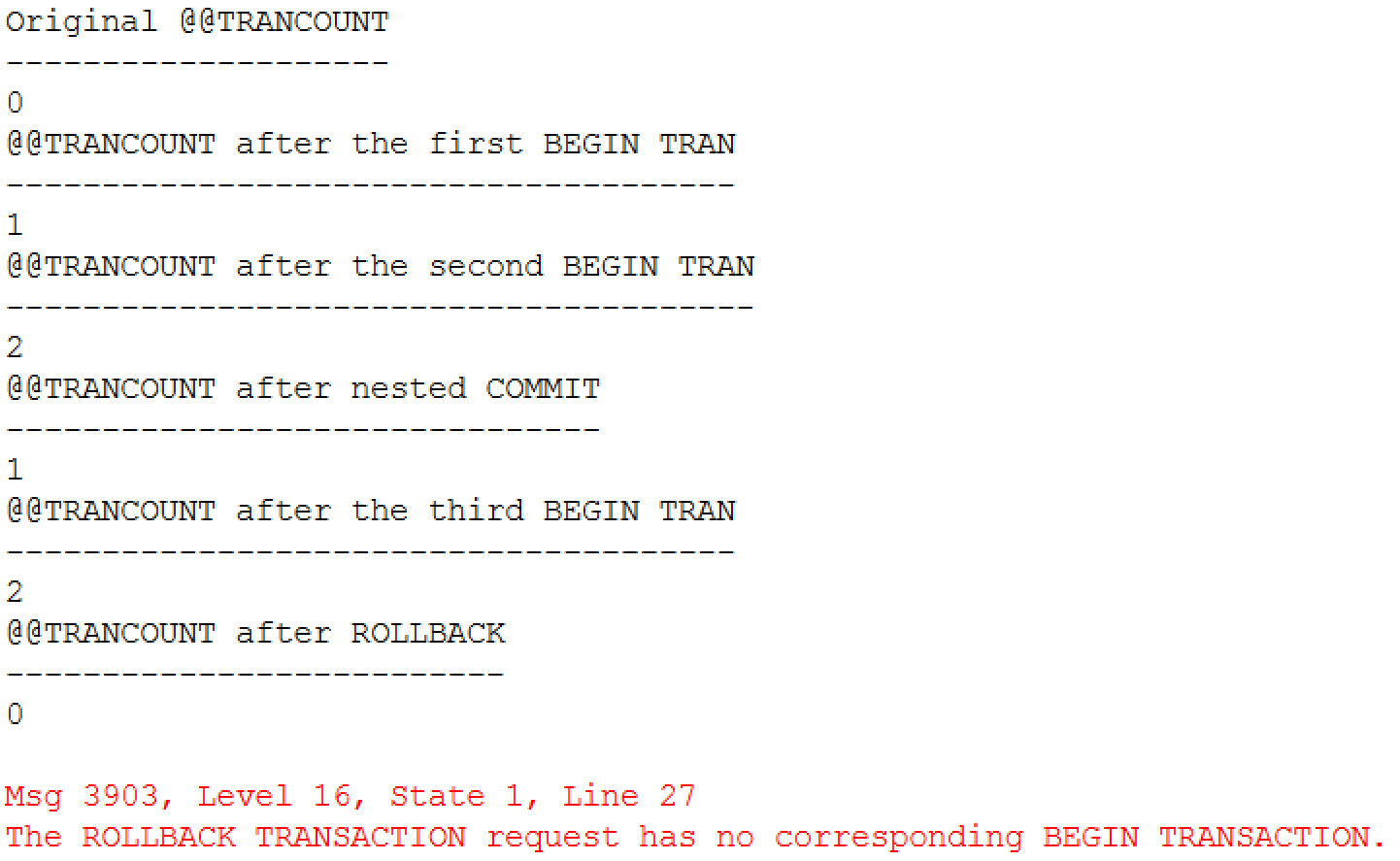
07. Nested Transactions

You can save the state of transaction and create a savepoint by using SAVE TRANSACTION statement. This will allow you to partially rollback a transaction returning to the most recent savepoint. The transaction will remain active and needs to be completed with explicit COMMIT or ROLLBACK statement later.

It is worth noting that uncommittable transactions with XACT_STATE() = -1 cannot be rolled back to savepoint. In practice, it means that you cannot rollback to savepoint after an error if XACT_ABORT is set to ON.

The code below illustrates savepoints in action. The stored procedure creates the savepoint when it runs in active transaction and rolls back to this savepoint in case of committable error.

create proc dbo.TryDeleteCustomer
(
    @CustomerId int 
)
as
begin
    -- Setting XACT_ABORT to OFF for rollback to savepoint to work
    set xact_abort off

    declare
        @ActiveTran bit

    -- Check if SP is calling in context of active transaction
    set @ActiveTran = IIF(@@TranCount > 0, 1, 0);

    if @ActiveTran = 0
        begin tran;
    else 
        save transaction TryDeleteCustomer;

    begin try
        delete dbo.Customers where CustomerId = @CustomerId;

        if @ActiveTran = 0
            commit;
        return 0;
    end try
    begin catch
        if @ActiveTran = 0 or XACT_STATE() = -1
        begin
            -- Rollback entire transaction
            rollback tran; 
            return -1; 
        end
        else begin
                -- Rollback to savepoint 
            rollback tran TryDeleteCustomer; 
            return 1; 
        end
    end catch;
end;
go

-- Test
declare
    @ReturnCode int

exec dbo.ResetData; 

begin tran
    exec @ReturnCode = TryDeleteCustomer @CustomerId = 1;
    select 
        1 as [CustomerId]
        ,@ReturnCode as [@ReturnCode]
        ,XACT_STATE() as [XACT_STATE()];
    
    if @ReturnCode >= 0
    begin
        exec @ReturnCode = TryDeleteCustomer @CustomerId = 2;
        select 
            2 as [CustomerId]
            ,@ReturnCode as [@ReturnCode]
            ,XACT_STATE() as [XACT_STATE()];    
    end
if @ReturnCode >= 0
    commit;
else 
    if @@TRANCOUNT > 0
        rollback;
go

select * from dbo.Customers;

The test triggered foreign key violation during the second dbo.TryDeleteCustomer call. This is non-critical error and, therefore, the code is able to commit after it as shown in Figure 8.

08. Transaction Has Been Committed After Rollback to Savepoint

It is worth noting that this example is shown for demonstration purposes only. From efficiency standpoint, it would be better to validate referential integrity and existence of the orders before deletion occurred rather than catching exception and rolling back to savepoint in case of an error.

I hope that those examples provided you the good overview of transaction management and error handling strategies in the system. If you want to dive deeper, I would strongly recommend you to read the great article by Erland Sommarskog, which provides you much more details on the subject.

Source code is available for download.

Table of Context

Implementing Sliding Windows Data Purge Pattern with Columnstore Indexes

It’s been a while since my last blog post. Many things happened, including another great PASS Summit where I presented the session of Data Partitioning (by the way, you can download the slides and demos from my Presentation page). As usual, I ran out of time 🙂

As many of you know, Data Partitioning is very big and complex subject, which is impossible to cover even with half-day session. One of the topics I left out of scope is how it plays with columnstore indexes. Even though partitioned columnstore tables are similar to B-Tree ones, there are some differences between them.

The biggest difference resides in partition function split and merge behavior. With B-Tree indexes, you can split and merge non-empty partitions. SQL Server would split or merge the data automatically, granted with the schema-modification (Sch-M) table lock held in place. Other sessions would be unable to access the table but at least split and merge would work.

This is not the case with columnstore indexes where you would get the error when you try to split or merge non-empty partitions. There are several reasons for this limitation. Without diving very deep into columnstore index internals, I could say that the only option of doing split of merge internally is rebuilding columnstore index on affected partitions. Fortunately, you can split and merge empty columnstore partitions, which allow you to workaround the limitation and also implement Sliding Window pattern and use partitioning to purge the data.

The Sliding Window pattern stands for scenario when we want to retain the data for some period of time. Consider the situation when we need to keep last 12 months of data. In the beginning of each month, we may purge the data that is older than 12 months, basically having a window on the data that slides purging the oldest data, based on a given schedule.

Data partitioning is great in this scenario. It allows to keep the purge process on metadata- and minimally logged-levels by switching the old-data partition to staging table truncating it afterwards. This helps to avoid log-intensive DELETE operations and reduce blocking in the system.

Let’s look at implementation. First, I would create partition function and scheme considering that now is November 2017 and we would need to retain 12-month of data starting November 2016.

create partition function pfOrders(datetime2(0))
as range right for values
('2016-11-01','2016-12-01','2017-01-01','2017-02-01'
,'2017-03-01','2017-04-01','2017-05-01','2017-06-01'
,'2017-07-01','2017-08-01','2017-09-01','2017-10-01'
,'2017-11-01','2017-12-01','2018-01-01');

create partition scheme psOrders 
as partition pfOrders
all to ([Primary]);

This code will create 16 partitions. The left-most partition will host the data prior 2016-11-01 and it will be empty. The two right-most partitions will host the data for December 2017 and everything starting on 2018-01-01. They also will be empty at this point.

There is the simple reason why we want to have two right-most partitions empty. Let’s assume that we will run the monthly purge process in December and December’s partition will already store some data. As part of the purge process, we would like to create the new partition for the “next month” data. It is beneficial to perform this and split partition function on empty partition. With B-Tree tables, it is nice to have implementation. It allows to avoid any data scans and movements reducing the time for schema modification lock being held. For columnstore indexes, this is actually the must have part of design – you would be unable to split non-empty partition at all.

If you ever implemented Sliding Window pattern with B-Tree indexes, you would be aware of empty right-most partition. However, you might notice that in our example, there is also empty left-most partition present. As I already mentioned, columnstore indexes would not allow you to merge non-empty partitions and you need to have an extra empty partition to perform the merge after old data is purged.

Let’s look at the process in details. As the first step, I will create two tables that will share the partition function and scheme. We will populate them with some data and create the columnstore indexes on the tables.

create table dbo.Orders
(
	OrderDate datetime2(0) not null,
	OrderId int not null,
	Placeholder char(100),
)
on psOrders(OrderDate);

create table dbo.OrderLineItems
(
	OrderDate datetime2(0) not null,
	OrderId int not null,
	OrderLineItemId int not null,
	Placeholder char(100),
)
on psOrders(OrderDate);

-- Left-most and right-most are empty
;with N1(C) as (select 0 union all select 0) -- 2 rows
,N2(C) as (select 0 from N1 as t1 cross join N1 as t2) -- 4 rows
,N3(C) as (select 0 from N2 as t1 cross join N2 as t2) -- 16 rows
,N4(C) as (select 0 from N3 as t1 cross join N3 as t2) -- 256 rows
,N5(C) as (select 0 from N4 as t1 cross join N4 as t2) -- 65,536 rows
,Ids(Id) as (select row_number() over (order by (select null)) from N5)
insert into dbo.Orders(OrderDate, OrderId)
	select dateadd(day,Id % 390,'2016-11-01'), ID
	from Ids;

insert into dbo.OrderLineItems(OrderDate,OrderId, OrderLineItemId)
	select OrderDate, OrderId, OrderId
	from dbo.Orders;

create clustered columnstore index CCI_Orders on dbo.Orders
on psOrders(OrderDate);

create clustered columnstore index CCI_OrderLineItems on dbo.OrderLineItems
on psOrders(OrderDate);

The next listing returns data distribution and allocation information for dbo.Orders table.

select 
	t.object_id, i.index_id, i.name as [Index], p.partition_number,
	p.[Rows], p.data_compression_desc, 
	fg.name as [Filegroup],
	sum(a.total_pages) as TotalPages, 
	sum(a.used_pages) as UsedPages, 
	sum(a.data_pages) as DataPages,
	sum(a.total_pages) * 8 as TotalSpaceKB, 
	sum(a.used_pages) * 8 as UsedSpaceKB, 
	sum(a.data_pages) * 8 as DataSpaceKB
from 
	sys.tables t with (nolock) join sys.indexes i with (nolock) on
		t.object_id = i.object_id
	join sys.partitions p with (nolock) on 
		i.object_id = p.object_id AND i.index_id = p.index_id
	join sys.allocation_units a with (nolock) on 
		p.partition_id = a.container_id
	join sys.filegroups fg with (nolock) on 
		a.data_space_id = fg.data_space_id
where
	t.object_id = object_id(N'dbo.Orders')
group by
	t.object_id, i.index_id, i.name, p.partition_number,
	p.[Rows], p.data_compression_desc, fg.name
order by 
	i.index_id, p.partition_number;

Figure 1 illustrates the output of the listing. As you can see, data is distributed across 13 partitions with left-most and two right-most partitions empty.

01. Data Distribution And Allocation Information

Let’s try to split non-empty partition, just for the demo purposes

alter partition scheme psOrders next used [Primary];

alter partition function pfOrders()
split range ('2017-11-15');

As expected, it would not work with the error message shown below.

02.Split Non-Empty Partition

The merge of non-empty partition would also fail.

03.Merge Non-Empty Partition

Fortunately, we can split an empty partition. Again, let’s assume that we want to start purging process in December.  I would insert a couple rows to December’s partitions making them non-empty.

insert into dbo.Orders(OrderDate, OrderId) values('2017-12-02',100000);
insert into dbo.OrderLineItems(OrderDate,OrderId, OrderLineItemId) values('2017-12-02',100000,100000);

Let’s create another empty partition by splitting partition function. The right-most partition is still empty and operation would succeed. As result, we will have separate empty partitions for January, 2018 and another partition that will store all data starting 2018-02-01. We will split the right-most empty partition again during our January’s 2018 purge process.

alter partition scheme psOrders next used [Primary];

alter partition function pfOrders()
split range ('2018-02-01');

The process of purging old data would consist of several steps. First, we need to create the staging tables to which we will switch old November 2016 partitions. Those tables need to be empty, have exactly the same schema with the main tables and reside on the same filegroup.

create table dbo.OrdersTmp
(
	OrderDate datetime2(0) not null,
	OrderId int not null,
	Placeholder char(100),
) on [Primary];

create clustered columnstore index CCI_OrdersTmp on dbo.OrdersTmp
on [Primary];

create table dbo.OrderLineItemsTmp
(
	OrderDate datetime2(0) not null,
	OrderId int not null,
	OrderLineItemId int not null,
	Placeholder char(100),
)
on [Primary];

create clustered columnstore index CCI_OrderLineItemsTmp on dbo.OrderLineItemsTmp
on [Primary];

After tables were created, we can switch November 2016 partitions there truncating staging tables afterwards. Remember that in the main tables, November 2016 is the second left-most partition.

alter table dbo.Orders switch partition 2 
to dbo.OrdersTmp;

alter table dbo.OrderLineItems switch partition 2 
to dbo.OrderLineItemsTmp;

truncate table dbo.OrdersTmp;
truncate table dbo.OrderLineItemsTmp;

If you look at dbo.Orders allocation information again, you would see that two left-most partitions are now empty as shown in Figure 4

04. Data Distribution And Allocation Information After Purge

Now they can be merged, which will complete our implementation.

alter partition function pfOrders()
merge range('2016-11-01');

As you can see, implementation of Sliding Window pattern with columnstore indexes is very similar to B-Tree tables. The only differences are:

  • You must have empty right-most partition pre-allocated to perform the split. I’d like to reiterate that even though it is not required with B-Tree indexes, such empty partition would reduce I/O overhead and table locking during split operation there.
  • You must have another empty left-most partition to perform the merge. This is not required nor needed with B-Tree indexes.

I’d like to thank Ned Otter (blog) for his suggestions and feedback. They convinced me to blog on the subject.

Source code is available for download.

Next (2017-11-29): Splitting and Merging Non-Empty Partitions in Columnstore Indexes

Compressing LOB (XML) Data in the Database

Some time ago we have discussed the several techniques that can help reducing the database size. I have received quite a few responses on that post and several people asked if I could provide more details and examples. Today I will try to follow up on one of the methods, such as reducing the size of LOB data (in particular XML) in the database.

As you know, SQL Server stores the data in regular B-Tree indexes in three different sets of the data pages called allocation units. The main data row structure and fixed-length data are stored in IN-ROW data pages. Variable-length data greater than 8,000 bytes in size is stored in LOB (large object) pages. Such data includes (max) columns, XML, CLR UDT and a few other data types. Finally, variable-length data, which does not exceed 8,000 bytes, is stored either in IN-ROW data pages when it fits into the page, or in ROW-OVERFLOW data pages. You can read more about it in the previous post and here.

Enterprise Edition of SQL Server allows you to reduce the size of the data by implementing data compression. However, data compression is applied to IN-ROW data only and it does not compress ROW-OVERFLOW and LOB data. Any large objects that do not fit into IN-ROW data pages remain uncompressed.

Unfortunately, there is very little we can do to reduce the size of the LOB data. SQL Server does not provide any build-in functional to address it. The only remaining option is compressing it manually – either on the client or with CLR routines. Obviously, compression and decompression adds overhead and, from SQL Server load standpoint, it is preferable to do it on the client side. However, in the large number of cases, you will need to access compressed data from T-SQL, and CLR integration is the only choice. Ideal implementation in that case would combine compression and decompression code in both tiers and use CLR only when it is necessary.

Fortunately, .Net implementation of the compression code is very simple and can be done with DeflateStream or GZipStream classes. Below you can see the code of CLR functions that perform compression and decompression. You can also download entire project with the link at the end of the post.

/// <summary>
/// Compressing the data
/// </summary>
[Microsoft.SqlServer.Server.SqlFunction(IsDeterministic = true, IsPrecise = true,
        DataAccess = DataAccessKind.None)]
public static SqlBytes BinaryCompress(SqlBytes input)
{
    if (input.IsNull)
        return SqlBytes.Null;

    using (MemoryStream result = new MemoryStream())
    {
        using (DeflateStream deflateStream = 
            new DeflateStream(result, CompressionMode.Compress, true))
        {
            deflateStream.Write(input.Buffer, 0, input.Buffer.Length);
            deflateStream.Flush();
            deflateStream.Close();
        }
        return new SqlBytes(result.ToArray());
    } 
}

/// <summary>
/// Decompressing the data
/// </summary>
[Microsoft.SqlServer.Server.SqlFunction(IsDeterministic = true, IsPrecise = true,
        DataAccess = DataAccessKind.None)]
public static SqlBytes BinaryDecompress(SqlBytes input)
{
    if (input.IsNull)
        return SqlBytes.Null;
    
    int batchSize = 32768;
    byte[] buf = new byte[batchSize];

    using (MemoryStream result = new MemoryStream())
    {
        using (DeflateStream deflateStream = 
            new DeflateStream(input.Stream, CompressionMode.Decompress, true))
        {
            int bytesRead;
            while ((bytesRead = deflateStream.Read(buf, 0, batchSize)) > 0)
                result.Write(buf, 0, bytesRead);
        }
        return new SqlBytes(result.ToArray());
    } 
}

You can define the functions in the database with the following code (you either need to get byte sequence of the compiled assembly from the demo script or compile CLR project).

create assembly LOBCompress
authorization dbo
from /*..*/
go

create function dbo.BinaryCompress(@input varbinary (max))
returns varbinary (max)
as external name [LOBCompress].[Compress].[BinaryCompress];
go

create function dbo.BinaryDecompress(@input varbinary (max))
returns varbinary (max)
as external name [LOBCompress].[Compress].[BinaryDecompress];
go

Now let’s see the process in action, create the test table and populate it with some data.

create table dbo.DataWithXML
(
    ID int not null,
    Data xml not null,

    constraint PK_DataWithXML
    primary key clustered(ID)
)
go

declare
    	@X xml

select @X = 
    (
        select *
        from master.sys.objects
        for xml raw, root('Data')
    )

;with n1(c) as (select 0 union all select 0) -- 2 rows
,n2(c) as (select 0 from n1 as t1 cross join n1 as t2) -- 4 rows
,n3(c) as (select 0 from n2 as t1 cross join n2 as t2) -- 16 rows
,n4(c) as (select 0 from n3 as t1 cross join n3 as t2) -- 256 rows
,n5(c) as (select 0 from n4 as t1 cross join n3 as t2) -- 4,096 rows
,ids(id) as (select row_number() over (order by (select null)) from n5)
insert into dbo.DataWithXML(ID,Data)
    select id, @X
    from Ids;

update dbo.DataWithXML
set Data.modify('replace value of (/Data/row/@object_id)[1]
with sql:column("ID")');

Let’s examine the size of the table and average size of XML there using the following queries:

select 
    index_id, partition_number, alloc_unit_type_desc
    ,index_level
    ,page_count
    ,page_count * 8 / 1024 as [Size MB]
from 
    sys.dm_db_index_physical_stats
    (
        db_id() /*Database */
        ,object_id(N'dbo.DataWithXML') /* Table (Object_ID) */
        ,1 /* Index ID */
        ,null /* Partition ID – NULL – all partitions */
        ,'detailed' /* Mode */
    )
go

select avg(datalength(Data)) as [Avg XML Size]
from dbo.DataWithXML;

As you can see in Figure 1, LOB allocation units are using 96MB of space to store the data. The average size of the XML data is 20,897 bytes per row. It is also worth mentioning that actual storage size for XML is 3 data pages per row, which is 24,576 bytes.

1. Uncompressed data: Storage space and XML Size

Let’s see what we can achieve by using compression. The code below creates another table and copies the data there, compressing it on the fly. As you see, the data is stored in varbinary(max) column.

create table dbo.DataWithCompressedXML
(
    ID int not null,
    Data varbinary(max) not null,

    constraint PK_DataWithCompressedXML
    primary key clustered(ID)
)
go

insert into dbo.DataWithCompressedXML(ID,Data)
    select ID, dbo.BinaryCompress(convert(varbinary(max),Data))
    from dbo.DataWithXML

Let’s check the size of the data in compressed table:

select avg(datalength(Data)) as [Uncompressed] 
from dbo.DataWithXML;

select avg(datalength(Data)) as [Compressed] 
from dbo.DataWithCompressedXML
go

select 
    index_id, partition_number, alloc_unit_type_desc
    ,index_level
	,page_count
	,page_count * 8 / 1024 as [Size MB]
from 
    sys.dm_db_index_physical_stats
    (
        db_id() /*Database */
        ,object_id(N'dbo.DataWithCompressedXML') /* Table (Object_ID) */
        ,1 /* Index ID */
        ,null /* Partition ID – NULL – all partitions */
        ,'detailed' /* Mode */
    )

As you can see in Figure 2, we were able to reduce the size of the table from 96 to 10MB decreasing the size of the XML in every row from 20,897 to 2,674 bytes.

2. Compressed data: Storage size and compressed XML size

It is also worth noting that in our case, the size of compressed data is less than 8,000 bytes and SQL Server was able to accommodate all the data using IN-ROW allocation units. Even though the new table is almost 10 times smaller than the old one, it has significantly more IN-ROW data pages in the index. This could introduce some performance side effects in some cases. For example, when system has poorly optimized queries that perform clustered index scans. Again, it could become the issue only if compressed data is less than 8,000 bytes. Otherwise, SQL Server will still store it using the LOB data pages.

Obviously, this implementation requires schema and code changes. We can mitigate it a little bit by abstracting it with the views as it is shown below.

create view dbo.vDataWithXML(ID, Data)
as
    select ID, convert(xml,dbo.BinaryDecompress(Data))
    from dbo.DataWithCompressedXML

We can even create INSTEAD OF trigger (yuck!) on the view to minimize the changes if absolutely needed.

Speaking of the overhead, compressing and decompressing are CPU intensive and there is the performance penalty of calling CLR functions. It is not that noticeable when you need to decompress the single or very few rows; however, it could be very significant on the large data sets. For example, when you need to decompress and shred XML and use some of its elements in a where clause of the query. The code below shows such an example.

set statistics time on
select count(*) 
from dbo.DataWithXML 
where Data.value('(/Data/row/@object_id)[1]','int') = 3;

select count(*) 
from dbo.vDataWithXML 
where Data.value('(/Data/row/@object_id)[1]','int') = 3;
set statistics time off

The second SQL that accesses the compressed table has to decompress XML for every row in the table. The execution times of the statements on my laptop are 116ms and 6,899ms respectively. As you see, the compression definitely comes at cost.

One of the ways to reduce such an overhead, is storing XML elements that are used in the queries in the separate table columns. Unfortunately, by-the-book approach with persisted calculated columns would not always works. It is possible to create and persist such a column using user-defined functions; however, SQL Server would ignore it in some cases. The code below shows the example that creates calculated column that contains the attribute we are using in our queries.

create function dbo.fnGetCompressedObjectId(@Compressed varbinary(max))
returns int
with schemabinding
as
begin
    return (convert(xml,dbo.BinaryDecompress(@Compressed))
                .value('(/Data/row/@object_id)[1]','int'))
end
go	 

alter table dbo.DataWithCompressedXML
add
    ObjId as dbo.fnGetCompressedObjectId(Data)
        persisted
go

-- It is a good practice to rebuild index after alteration
alter index PK_DataWithCompressedXML 
on dbo.DataWithCompressedXML rebuild
go

alter view dbo.vDataWithXML(ID, Data, ObjId)
as
    select ID, convert(xml,dbo.BinaryDecompress(Data)), ObjId
    from dbo.DataWithCompressedXML
go

Unfortunately, if you ran the following query: select count(*) from dbo.vDataWithXML where ObjId = 3, you’d notice that SQL Server recalculates the value of the calculated column even though it is persisted and functions are defined as deterministic and precise. This is just the limitation of the Query Optimizer. Figure 3 shows that ObjId is recalculated.

3. Execution plan of the query

There is still the possibility of using persisted calculated columns. For example, you can define CLR function, which decompress and parse XML and return ObjID as the integer. Something like that:

.Net CLR:
[Microsoft.SqlServer.Server.SqlFunction(IsDeterministic = true, IsPrecise = true,
            DataAccess = DataAccessKind.None)]
public static SqlInt32 GetObjId(SqlBytes input)
{
    if (input.IsNull)
        return SqlInt32.Null;
    /* Parsing XML with XmlReader and return ObjId attribute */
}

SQL: 
create function dbo.GetObjId(@input varbinary (max))
returns int
as external name [LOBCompress].[Compress].[GetObjId]
go

alter table dbo.DataWithCompressedXML drop column ObjId
go

alter table dbo.DataWithCompressedXML
add
    ObjId as dbo.GetObjId(Data)
        persisted
go

alter index PK_DataWithCompressedXML 
on dbo.DataWithCompressedXML rebuild
go

Now, if you run the previous query: select count(*) from dbo.vDataWithXML where ObjId = 3, it would work just fine and does not recalculate the column value. Figure 4 shows the execution plan in this case.

4. Execution plan that utilizes calculated column

It is worth mentioning that execution time of this query on my laptop is just 3 milliseconds comparing to 116 milliseconds of the query against dbo.DataWithXML table. The query is significantly faster because it does not need to shred XML to obtain ObjID value.

Obviously, creating separate CLR methods for each calculated column can lead to some coding overhead. You can consider using regular columns instead and populate them in the code or even in the triggers. Each approach has the own set of benefits and downsides based on the use-cases implemented in the system.

Compressing LOB data in the database could help you to significantly reduce the database size in the large number of cases. However, it adds an overhead of compressing and decompressing data. In some cases, such overhead would be easily offset by the smaller data size, less I/O and buffer pool usage but in any case, you should be careful and take all other factors into the consideration.

Source code is available for download.

Optimizing Substring Search Performance in SQL Server

The requirement of searching data by part of the value is very common in business applications. All of us are familiar with it – users want to be able to search by entering just a few letters from the client or article name; locate postal address by typing just a part of the street; or do something similar in dozens of the other cases.

Obviously, there are many ways to skin the cat and implement such a search. In some complex and performance-critical cases we can use external to SQL Server solutions, for example Apache Lucene. In others, we can use Full-Text Search or even do the brute force approach with LIKE operator. Today, I would like to talk about the latter one. After all, even though LIKE is not necessarily the fastest solution, its performance could often be acceptable especially with relatively small tables. Last but not least, it comes with very little implementation cost.

Unfortunately, LIKE operator cannot use Index Seek unless you are performing the prefix search. In that case, when you are searching by the beginning of the string – for example, LastName LIKE ‘Smit%’ condition – SQL Server is able to locate subset of the data where predicate needs to be evaluated. In our example, the predicate, in the nutshell, is the following condition: LastName >= ‘Smit’ and LastName < ‘Smiu’, which is perfectly SARGable and suitable for the fast Index Seek.

This is not the case, however, when LIKE expression requires SQL Server to find patterns in the middle of the string – for example, in LastName LIKE ‘%Smit%’ situation. The only option for SQL Server is evaluating expression against every row from the index, which leads to the Index Scan.

As strange as it sounds, you can often improve search performance by challenging business requirements. Even though customers want to be able to search by substring, in the very large number of cases prefix search would do. For example, when you are calling customer service somewhere and asking them to look up your account, you’d usually provide them the first few letters of your name rather than some letters from the middle of it.

Unfortunately, changing the business requirements is not always possible. In some cases, we do not have any choices but implementing substring search. In those occasions, there are two ways to improve the performance – reduce the number of rows where LIKE predicate must be evaluated and reduce predicate evaluation time.

Reducing the number of rows for predicate evaluation greatly depends on the indexes. While you cannot do much when LIKE is the only predicate in the query, such condition is usually an exception rather than the rule. In case when query has multiple predicates, the right composite indexes would help. The key here is adding evaluation column as the key or included column of the index and avoiding post-Key Lookup predicate evaluation.

For example, consider multi-tenant shopping cart system and the query that need to return the list of the articles that belong to particular tenant. The query could be implemented as follows:

select ..
from dbo.Articles
where TenantID = @TenantID and Name LIKE '%' + @paramName + '%'
order by Name

Such query would benefit from the following index, which will limit LIKE predicate evaluation to the single tenant scope. As the side note, adding Name as the key rather than included column would help to avoid SORT operator in the execution plan – data in the index would be sorted according to order by clause of the query.

create index IDX_Articles_TenantID_Name
on dbo.Articles(TenantID,Name)

Reducing the predicate evaluation time is the trickier subject. Fortunately, you can often achieve significant performance increase by utilizing binary collations during such an evaluation.

Let’s take a look at the example. As the first step, we will create a table and populate it with some random data. Col1, Col2 and Col3 columns are populated with randomly generated GUIDs and VarCol and NVarCol store concatenated values from them using SQL_Latin1_General_CP1_CI_AS collations. Finally, I am creating nonclustered indexes on VarCol and NVarCol columns to minimize amount of data pages SQL Server need to read during our tests and make those tests consistent.

create table dbo.Data
(
    ID int not null,
    Col1 uniqueidentifier not null
        default NEWID(),
    Col2 uniqueidentifier not null
        default NEWID(),
    Col3 uniqueidentifier not null
        default NEWID(),
    VarCol varchar(108) null,
    NVarCol nvarchar(108) null,
    
    constraint PK_Data
    primary key clustered(ID)
)
go

;with N1(C) as (select 0 union all select 0) -- 2 rows
,N2(C) as (select 0 from N1 as T1 cross join N1 as T2) -- 4 rows
,N3(C) as (select 0 from N2 as T1 cross join N2 as T2) -- 16 rows
,N4(C) as (select 0 from N3 as T1 cross join N3 as T2) -- 256 rows
,N5(C) as (select 0 from N4 as T1 cross join N4 as T2) -- 65,536 rows
,IDs(ID) as (select row_number() over (order by (select NULL)) from N5)
insert into dbo.Data(ID)
    select ID from IDs;

update dbo.Data
set
    VarCol =
        convert(varchar(36),Col1) +
        convert(varchar(36),Col2) +
        convert(varchar(36),Col3)
    ,NVarCol =
        convert(nvarchar(36),Col1) +
        convert(nvarchar(36),Col2) +
        convert(nvarchar(36),Col3)
go

create nonclustered index IDX_Data_VarCol
on dbo.Data(VarCol);

create nonclustered index IDX_Data_NVarCol
on dbo.Data(NVarCol);

Next, let’s randomly choose substring to search using one of the rows from the table. You would obviously have different data in your case/

select * from dbo.Data where ID = 10000

01. Choosing test substring for the search.

Now, let’s run SELECT statements that perform substring search against both columns and measure the execution time of the selects. I am disabling parallelism with MAXDOP 1 hint to avoid any parallelism overhead during queries execution.

declare
    @V varchar(32) = '9D81AB12'
    ,@NV nvarchar(32) = N'9D81AB12'

set statistics time on

select count(*)
from dbo.Data
where VarCol like '%' + @V + '%'
option (maxdop 1);

select count(*)
from dbo.Data
where NVarCol like '%' + @NV + '%'
option (maxdop 1);

set statistics time off

In my environment, CPU times of the first and second statements are 203 and 844 milliseconds respectively. Obviously, you would get the different results in your system and performance would greatly depend on the data.

It is also worth mentioning, that index on NVarCol is about two times larger than index on VarCol column due to the fact, that unicode data uses 2-bytes per character to store the data as the opposite to 1-byte per character with non-unicode varchars. However, the overhead of the extra logical reads is minimal.

Now let’s measure execution time using binary collations. First, we will alter the table adding two calculated columns that represent our strings in binary collation and creating nonclustered indexes afterwards.

alter table dbo.Data
add VarColBin as upper(VarCol) collate Latin1_General_100_Bin2
persisted;

alter table dbo.Data
add NVarColBin as upper(NVarCol) collate Latin1_General_100_Bin2
persisted;

create nonclustered index IDX_Data_VarColBin
on dbo.Data(VarColBin);

create nonclustered index IDX_Data_NVarColBin
on dbo.Data(NVarColBin);

PERSISTED keyword tells SQL Server to materialize calculated columns and store them in the data row. Technically speaking, you do not need to persist calculated columns in our case – you can index them even when they are not persisted, which helps to avoid clustered index row size increase. However, you need to be careful making sure that SQL Server always uses nonclustered index for the search. Otherwise, search performance could be even slower than with nonbinary collation – SQL Server will need to calculate column values on the fly before evaluating LIKE predicate.

Another very important factor to remember is case sensitivity of the binary collation. You need to convert your data to upper or lower case if your system uses case-insensitive collation. Obviously, you need to use the same conversion rule for the search predicate.

declare
    @V varchar(32) = '9D81AB12'
    ,@NV nvarchar(32) = N'9D81AB12'

set statistics time on

select count(*)
from dbo.Data
where VarColBin like '%' + Upper(@V) + '%' collate Latin1_General_100_Bin2
option (maxdop 1);

select count(*)
from dbo.Data
where NVarColBin like '%' + Upper(@NV) + '%' collate Latin1_General_100_Bin2
option (maxdop 1);

set statistics time off

The execution times in my environment are 125 and 62 milliseconds respectively. You can see all the results in Figure 2 below.

02. Test results

As you can see, we got more than 13 times performance improvement in case of the unicode data. Performance improvement with non-unicode strings are less drastic; however, it still ran about 40% faster than before. It is also worth mentioning that with the binary collation, predicate evaluation against unicode data is faster than with varchar data. At least with my test data.

Lastly, the word of caution. While that technique can be help to improve performance of substring search and reduce CPU load in the system, you should not treat it as the replacement of the proper indexing. After all, you can get much better ROI by investing your time into query optimization. However, it is the great technique to use in conjunction with query optimization and index tuning when you need to get the most from your queries.

Plan Cache: Plan Reuse

Last time we have discussed how parameter sniffing can affect the quality of generated execution plans. Today, I would like to talk about another aspect of plan caching, which is plan reuse. Plans, cached by SQL Server, must be valid for any combination of parameters during future calls that reuse the plan. In some cases, this can lead to situations where a cached plan is suboptimal for a specific set of parameter values.

One of the common code patterns that leads to such situations is the implementation of stored procedure that search for the data based on a set of the optional parameters. Let’s look at the typical implementation of such stored procedure as shown in the code below. That code uses dbo.Employees table from the “parameter sniffing” post and it also creates two nonclustered indexes on that table.

create proc dbo.SearchEmployee
(
	@Number varchar(32) = null
	,@Name varchar(100) = null
)
as
begin
	select Id, Number, Name, Salary, Country
	from dbo.Employees
	where 
		((@Number is null) or (Number=@Number)) and
		((@Name is null) or (Name=@Name))
end
go

create unique nonclustered index IDX_Employees_Number
on dbo.Employees(Number);

create nonclustered index IDX_Employees_Name
on dbo.Employees(Name);

There are several different approaches how SQL Server can execute the query from the stored procedure based on what parameters were provided. In the large number of cases, the most efficient approach would be using Nonclustered Index Seek and Key Lookup operators. Let’s run the stored procedure several times with different parameter combinations and check the execution plans:

exec dbo.SearchEmployee @Number = '10000';
exec dbo.SearchEmployee @Name = 'Canada Employee: 1';
exec dbo.SearchEmployee @Number = '10000', @Name = 'Canada Employee: 1';
exec dbo.SearchEmployee @Number = NULL, @Name = NULL;

01.Execution Plans When Plans Are Cached

SQL Server compiles stored procedure at time of the first call when only @Number parameter was provided. Even though, the most efficient execution plan for this case is IDX_Employees_Number Index Seek operation, SQL Server cannot cache such execution plan because it would not be valid for the case, when @Number parameter is NULL. Therefore, SQL Server generated and cached execution plan that utilizes Index Scan operation, which is highly inefficient in case, when @Number parameter is not provided. In that case, SQL Server performs Key Lookup operation for every row in the nonclustered index optionally evaluating predicate on @Name parameter afterwards.

Similar to parameter sniffing issues, you can address this problem with statement-level recompilation as it is shown below. SQL Server recompiles the query on every call, and therefore it can choose the most beneficial execution plan for every parameter set.

It is also worth mentioning that the plans are not cached in cases where statement-level recompile is used.

alter proc dbo.SearchEmployee
(
	@Number varchar(32) = null
	,@Name varchar(100) = null
)
as
begin
	select Id, Number, Name, Salary, Country
	from dbo.Employees
	where 
		((@Number is null) or (Number=@Number)) and
		((@Name is null) or (Name=@Name))
	option (recompile)
end

02.Execution Plans With Statement-Level Recompile

As we already discussed, query recompilation adds CPU overhead. That overhead can be acceptable in case of large and complex queries when compilation time is just the fraction of the query execution time and system is not CPU-bound. In that case, recompilation can even help producing the better execution plans, which would be generated based on the current parameter values, especially if table variables are involved. However, this recompilation overhead is usually not acceptable in case of OLTP queries that are called very often.

One of the options you can use to address the issue is writing multiple queries using IF statements covering all possible combinations of parameters. SQL Server would cache the plan for each statement in the procedure. Listing below shows such an approach, however it quickly becomes unmanageable with a large number of parameters. The number of combinations to cover is equal to the number of parameters squared.

alter proc dbo.SearchEmployee
(
	@Number varchar(32) = null
	,@Name varchar(100) = null
)
as
begin
	if @Number is null and @Name is null
		select Id, Number, Name, Salary, Country
		from dbo.Employees
	else if @Number is not null and @Name is null
		select Id, Number, Name, Salary, Country
		from dbo.Employees
		where Number=@Number
	else if @Number is null and @Name is not null
		select Id, Number, Name, Salary, Country
		from dbo.Employees
		where Name=@Name
	else 
		select Id, Number, Name, Salary, Country
		from dbo.Employees
		where Number=@Number and Name=@Name
end

In the case of a large number of parameters, dynamic SQL becomes the only option. SQL Server will cache the execution plans for each dynamically generated SQL statement. Remember that using dynamic SQL breaks ownership chaining, and it always executes in the security context of CALLER. You should also always use parameters with dynamic SQL to avoid SQL Injection.

alter proc dbo.SearchEmployee
(
	@Number varchar(32) = null
	,@Name varchar(100) = null
)
as
begin
	declare
		@SQL nvarchar(max) = N'	
select Id, Number, Name, Salary, Country
from dbo.Employees
where 1=1'
	
	if @Number is not null
		select @Sql = @SQL + N' and Number=@Number'
	if @Name is not null
		select @Sql = @SQL + N' and Name=@Name'
	exec sp_executesql @Sql, N'@Number varchar(32), @Name varchar(100)'
		,@Number=@Number, @Name=@Name
end

While most of us are aware about danger of using optional parameters and OR predicates in the queries, there is another less known issue associated with filtered indexes. SQL Server will not generate and cache a plan that uses a filtered index, in cases when that index cannot be used with some combination of parameter values.

Listing below shows an example. SQL Server will not generate the plan, which is using the IDX_RawData_UnprocessedData index, even when the @Processed parameter is set to zero because this plan would not be valid for a non-zero @Processed parameter value.

create unique nonclustered index IDX_RawData_UnprocessedData
on dbo.RawData(RecID)
include(Processed)
where Processed = 0;

-- Compiled Plan for the query would not use filtered index
select top 100 RecId, /* Other columns */
from dbo.RawData
where RecID > @RecID and Processed = @Processed
order by RecID;

In that particular case, rewriting the query using IF statement would be, perhaps, the best option.

if @Processed = 0
	select top 1000 RecId, /* Other Columns */
	from dbo.RawData
	where RecId > @RecId and Processed = 0
	order by RecId;
else 
	select top 1000 RecId, /* Other Columns */
	from dbo.Data
	where RecId > @RecId and Processed = 1
	order by RecId;

Unfortunately, IF statement does not always help. In some cases, SQL Server can auto-parametrize the queries and replace some of the constants with auto-generated parameters. That behavior allows SQL Server to reduce the size of the plan cache; however, it could lead to all plan reuse issues we have already discussed.

By default, SQL Server uses SIMPLE parametrization and parametrize only the simple queries. However, if database or query are using FORCED parametrization, that behavior can become the issue. Let’s look at a particular example and create a database with a table with a filtered index and populate it with some data, as shown below.

use master
go

create database ParameterizationTest
go

use ParameterizationTest
go

create table dbo.RawData
(
	RecId int not null identity(1,1), 
	Processed bit not null, 
	Placeholder char(100),
	constraint PK_RawData
	primary key clustered(RecId)
);

/* Inserting:
	Processed = 1: 65,536 rows
	Processed = 0: 16 rows */
;WITH N1(C) AS (SELECT 0 UNION ALL SELECT 0) -- 2 rows
,N2(C) AS (SELECT 0 FROM N1 AS T1 CROSS JOIN N1 AS T2) -- 4 rows
,N3(C) AS (SELECT 0 FROM N2 AS T1 CROSS JOIN N2 AS T2) -- 16 rows
,N4(C) AS (SELECT 0 FROM N3 AS T1 CROSS JOIN N3 AS T2) -- 256 rows
,N5(C) AS (SELECT 0 FROM N4 AS T1 CROSS JOIN N4 AS T2 ) -- 65,536 rows
,IDs(ID) AS (SELECT ROW_NUMBER() OVER (ORDER BY (SELECT NULL)) FROM N5)
insert into dbo.RawData(Processed)
	select 1
	from Ids;

insert into dbo.RawData(Processed)
	select 0
	from dbo.RawData
	where RecId <= 16;

create unique nonclustered index IDX_RawData_Processed_Filtered 
on dbo.RawData(RecId)
include(Processed)
where Processed = 0;

For the next step, let’s run the queries that count a number of unprocessed rows in both SIMPLE and FORCED parametrization modes.

select count(*)
from dbo.RawData
where Processed = 0			
go

alter database ParameterizationTest set parameterization forced
go

select count(*)
from dbo.RawData
where Processed = 0

If you examine the execution plans shown in Figure 3, you will notice that SQL Server utilized a filtered index in the case of a SIMPLE parametrization. SQL Server can cache this plan because of the constant in the Processed=0 predicate. Alternatively, with FORCED parametrization, SQL Server parametrizes the query using the parameter in the Processed=@0 predicate. Therefore, it cannot cache the plan with the filtered index because it would not be valid for the case when a query selects processed (Processed=1) rows. SQL Server generated the execution plan with a Clustered Index Scan, which is far less efficient in this case.

03.Execution Plans and Parametrization

The workaround in this case is using SIMPLE parametrization for the database, or forcing it on query level with plan guide (more on it later). In some cases, you would also need to rewrite the query and use one of the constructs that prevent parametrization in SIMPLE parametrization mode, such as IN, TOP, DISTINCT, JOIN, UNION, subqueries and quite a few others.

Plan caching and plan reuse are the great features that help to reduce CPU load on the server. However, they introduce several side effects you need to be aware of and keep them in mind when you write queries and stored procedures.

Source code is available for download

Writing Triggers in the Right Way

The only correct way of writing triggers is not writing them. I would repeat – the only correct way of writing triggers is not writing them. Triggers negatively affect performance. AFTER triggers introduce fragmentation and increase tempdb load due to version store usage. Triggers are running in context of transaction, increase the time in which locks are held and contribute to locking and blocking in the system. However, in some cases, we have to use triggers and it is important to develop them correctly.

SQL Server fires triggers on statement rather than row level. For example, if update statement modified 10 rows, AFTER UPDATE and/or INSTEAD OF UPDATE trigger would fire once rather than 10 times. Therefore, trigger must handle situations when inserted and/or deleted tables have multiple rows.  Let’s look at the example and create a table with AFTER INSERT trigger as shown below:

create table dbo.Data 
( 
	ID int not null, 
	Value varchar(32) 
) 
go 

create trigger trgData_AI on dbo.Data 
after insert 
as 
	/* Some code */ 
	declare 
		@ID int 
	set @ID = (select ID from inserted) 
	/* Some code */

Everything is fine when you inserted a single row. However, multi-row insert would fail with exception shown below.

Msg 512, Level 16, State 1, Procedure trgData_AI, Line 9
Subquery returned more than 1 value. This is not permitted when the subquery follows =, !=, <, <= , >, >= or when the subquery is used as an expression.
The statement has been terminated.

And there is another consequence of statement-level nature of triggers. They fire even if DML statement did not modify any rows. Would it introduce any issues in the system or not depends on implementation. However, it would always lead to unnecessary performance overhead.

Let’s look at example. The code below creates another table and changes trigger in a way, that mimics behavior of audit functional, which is frequently implemented based on triggers.

create table dbo.Audit 
( 
	ID int not null identity(1,1), 
	OnDate datetime2(0) not null 
		constraint DEF_Audit_OnDate  
		default getutcdate(), 
	Message varchar(64) not null, 
)
go

alter trigger trgData_AI on dbo.Data 
after insert 
as 
begin
	declare 
		@Msg varchar(64) = 'Triggers are bad. And @@ROWCOUNT=' + convert(varchar(10),@@rowcount) 

	insert into dbo.Audit(Message) values(@Msg); 
end

Now let’s run insert statement, which does not insert any rows to the table.

insert into dbo.Data(ID, Value) 
	select 1, 'ABC'  
	where 1 = 0

If you checked content of Audit table, you would see that trigger was fired:

01. Content of Audit table

So the first important conclusion is that every trigger must checks @@ROWCOUNT variable as the very first statement in implementation.

SET NOCOUNT ON should be the second action trigger does. Without that SQL Server returns affected number of rows for each operator in the trigger in addition to original DML statement. Some client libraries rely on the single message in the output and would not work correctly in case of multiple messages. Therefore, the first two statements in the trigger should look like it is shown below.

alter trigger trgData_AI on dbo.Data 
after insert 
as 
begin
	if @@ROWCOUNT = 0
		return
	set nocount on

	/* Some Code Here */
end

Finally, there is another caveat. While implementation above works for insert, update and delete operators, it is not the case with merge@@ROWCOUNT in this case represents total number of rows affected by merge statement rather than by individual insert, update or delete action in the trigger. Let’s prove it with the example.

create table dbo.Data2(Col int not null)
go

create trigger trg_Data_AI on dbo.Data2
after insert 
as
	select 
		'After Insert' as [Trigger]
		,@@RowCount as [RowCount]
		,(select count(*) from inserted) as [Inserted Cnt]
		,(select count(*) from deleted) as [Deleted Cnt]
go

create trigger trg_Data_AU on dbo.Data2
after update
as
	select 
		'After Update' as [Trigger]
		,@@RowCount as [RowCount]
		,(select count(*) from inserted) as [Inserted Cnt]
		,(select count(*) from deleted) as [Deleted Cnt]
go

create trigger trg_Data_AD on dbo.Data2
after delete
as
	select 
		'After Delete' as [Trigger]
		,@@RowCount as [RowCount]
		,(select count(*) from inserted) as [Inserted Cnt]
		,(select count(*) from deleted) as [Deleted Cnt]
go

Now let’s run MERGE statement as shown below:

merge into dbo.Data2 as Target
using (select 1 as [Value]) as Source
on Target.Col = Source.Value
when not matched by target then
	insert(Col) values(Source.Value)
when not matched by source then
	delete
when matched then
	update set Col = Source.Value;

The table is empty, therefore only one insert statement would be executed. However, as you should see below, all three triggers were fired, It is worth mentioning that previous code example demonstrated very bad practice of returning result sets from trigger. You should avoid doing it in production code.

02. Triggers and MERGE statement

The right way to deal with such situation is checking content of inserted and deleted tables as shown below.

alter trigger trg_Data_AI on dbo.Data2
after insert 
as
	if @@rowcount = 0 
		return
	set nocount on
	if exists(select * from inserted)
		/* Some Code Here */      
go

alter trigger trg_Data_AU on dbo.Data2
after update
as
	if @@rowcount = 0 
		return
	set nocount on
	if	exists(select * from inserted) and 
		exists(select * from deleted)
		/* Some Code Here */      
go

alter trigger trg_Data_AD on dbo.Data2
after delete
as
	if @@rowcount = 0 
		return
	set nocount on
	if	exists(select * from deleted)
		/* Some Code Here */

I hope that those tips will help you to write trigger in the most optimal way. However, I would repeat – the best way of writing triggers is not writing them at all.

Unwinding Table Spools

One of the questions I have often been asked during various SQL Server events is what exactly Table Spool operator does in execution plan. I would try to answer it today.

Spool operators, in the nutshell, are internal in-memory or on-disk caches/temporary tables. SQL Server often uses spools for performance reasons to cache results of complex subexpressions that needs to be used multiple times during query execution.

Let’s look at the example and create the table, which stores some sales information as shown below:

create table dbo.Orders
(
    OrderID int not null,
    CustomerId int not null,
    Total money not null,
    constraint PK_Orders
    primary key clustered(OrderID)
);

;with N1(C) as (select 0 union all select 0) -- 2 rows
,N2(C) as (select 0 from N1 as T1 cross join N1 as T2) -- 4 rows
,N3(C) as (select 0 from N2 as T1 cross join N2 as T2) -- 16 rows
,N4(C) as (select 0 from N3 as T1 cross join N3 as T2) -- 256 rows
,Nums(Num) as (select row_number() over (order by (select null)) from N4)
    insert into dbo.Orders(OrderId, CustomerId, Total)
        select Num, Num % 10 + 1, Num
        from Nums;

Now let’s run the query that returns the list of orders with the information about total amount of sales on per-customer basis.

select OrderId, CustomerID, Total
	,Sum(Total) over(partition by CustomerID) as [Total Customer Sales] 
from dbo.Orders

As you see, in the execution plan below, SQL Server scans the table, sorts the data based on CustomerID order and uses Table Spool operator to cache the results. It allows SQL Server to access the cached data and avoid expensive sorting operation later.

01. Execution Plan with Spool operators

Even though Table Spool operator is shown in the execution plan multiple times, it is essential the same spool/cache. SQL Server builds it the first time and using its data later.

Technically speaking, there are two different logical spool operators – Eager Spool and Lazy Spool. The only difference between them are how data is populated. With Eager Spool, SQL Server fetches all rows as soon as spool is called. With Lazy Spool, SQL Server fetches rows on demand – when they are needed.

SQL Server also uses spools for Halloween Protection when modifying the data. Halloween Protection helps to avoid situations when data modifications affect what data need to be updated. The classic example of such situation is shown below. Without Halloween Protection, insert statement would fall into infinitive loop, reading rows it has been inserting.

create table dbo.HalloweenProtection
(
	Id int not null identity(1,1),
	Data int not null
);

insert into dbo.HalloweenProtection(Data)
	select Data from dbo.HalloweenProtection;

As you can see in the execution plan of insert statement, SQL Server uses Table Spool operator to cache the data from table as of before insert starts to avoid infinitive loop during execution.

02. Halloween Protection and Table Spools.

Halloween Protection has very interesting side-effect when we are talking about multi-statement user-defined functions (both, scalars and table-valued). Using multi-statement functions is bad practice by itself, however creating them without SCHEMABINDING option is even worse. That option forces SQL Server to analyze if user-defined function performs data access and avoid extra Halloween Protection-related Spool operators in the execution plan.

Let’s see the example and create two user-defined functions and using them in where clause of update statements.

create function dbo.ShouldUpdateData(@Id int)
returns bit
as
begin
	return (1)
end
go

create function dbo.ShouldUpdateDataSchemaBound(@Id int)
returns bit
with schemabinding
as
begin
	return (1)
end
go

update dbo.HalloweenProtection
set Data = 0
where dbo.ShouldUpdateData(ID) = 1;

update dbo.HalloweenProtection
set Data = 0
where dbo.ShouldUpdateDataSchemaBound(ID) = 1;

Neither of functions access the data and therefore can introduce Halloween effect. However, SQL Server does not know that in case of non-schema bound function and add Spool operator to execution plan as shown below.

03. Execution Plans for user-defined functions

Bottom line – you should always make functions schema-bound when you create them.

Spool temporary tables are usually referenced as worktables in I/O statistics for the queries. You should analyze table spool-related reads during query performance tuning. While spools can improve performance of the queries, there is the overhead introduced by unnecessary spools. You can often remove them by creating appropriate indexes on the tables.

Optimizing SQL Server Spatial Queries with Bounding Box

SQL Server supports two data types to store spatial information – geometry and geography. Geometry supports planar, or Euclidean, flat-earth data. Geography supports ellipsoidal round-earth surface. Both data types can be used to store location information, such as GPS latitude and longitude coordinates. Geography data type considers Earth roundness and provides slightly better accuracy although it has stricter requirements to the data. As a couple of examples, data must fit in the single hemisphere and polygons must be defined in specific ring orientation.

Storing location information in geometry data type introduces its own class of problems. It works fine and often has better performance than geography data type. Although, we cannot calculate the distance between points – the unit of measure for result is decimal degrees, which are useless in non-flat surface.

Let’s take a look at spatial data type performance in one of the specific use-cases, such as distance calculation between two points. Typical use-case for that scenario is the search for the point of interest (POI) close to specific location. First, let’s create three different tables storing POI information in the different format and populate them with some data.

01. Test tables

02. Populating test tables with data

The first table dbo.Locations stores the coordinates using decimal(9,6) data type. Two other tables are using geography data type. Finally, the table dbo.LocationsGeoIndexed has Location column indexed with special type of the index called spatial index. Those indexes help improving performance of some operations, for example distance calculation or check if objects are intersecting.

It is worth mentioning that the first table uses decimal(9,6) data type rather than float. This decision saves us six bytes per pair of values and provides the accuracy that exceed the accuracy of commercial-grade GPS receivers.

Let’s run the tests that measures performance of the queries that calculate the number of locations within one mile from Seattle City Center. In case of dbo.Locations table, we will use dbo.CalcDistanceCLR function, which we defined earlier. For two other tables we will call spatial method STDistance.

03. Test queries (table-wide lookup)

04. Execution plans (table-wide lookup)

The first and second queries perform clustered index scan and calculate the distance for every row from the table. Last query uses spatial index to lookup such rows. We can see execution times for the queries in the table below.

05. Execution time (Table-wide lookup)

As we see, spatial index greatly benefits the query. It is also worth mentioning, that without the index, performance of CalcDistanceCLR method is better comparing to STDistance.

Although spatial index greatly improves the performance, it has its own limitations. It works in the scope of entire table and all other predicates are evaluated after spatial index operations. That can introduce suboptimal plans in some cases.

As the example, let’s look at the use-case, when we store POI information on company-by-company basis .

06. Test table creation (company-wide lookup)

In case, when we perform POI lookup for specific company, CompanyId column must be included as the predicate to the queries. SQL Server has two choices how to proceed. The first choice is clustered index seek based on CompanyId value calling STDistance method for every POI that belongs to the company. Another choice is using spatial index, find all POIs within the specified distance regardless of what company they belong and, finally, join it with the clustered index data. Let’s run those queries.

07. Test queries (company-wide lookup)

Neither method is efficient in case when table stores the large amount of data for the large number of companies. Execution plan of the first query utilizing clustered index seek shows that it performed STDistance call 241,402 times – once per every company POI.

08. Execution plan (clustered index seek approach)

The execution plan for the second query shows that spatial index lookup returned 550 rows – all POI in the area, regardless of what company they belong. SQL Server had to join the rows with the clustered index before evaluating CompanyId predicate.

09. Execution plan (Spatial index approach)

One of the ways to solve such problem called Bounding Box approach. That method allows us to minimize the number of the calculations by filtering out POIs that are outside of the area of interest.

10. Bounding box

All points we need to select residing in the circle with location as the center point and radius specified by the distance. The only points we need to evaluate are residing within the box that inscribes that circle.

We can calculate the coordinates of the corner points of the box, persist it in the table and use regular non-clustered index to pre-filter the data. This would allow us to minimize the number of expensive distance calculations to perform.

Calculation of the bounding box corner points can be done with CLR table-valued function shown below.

11. Calculating bounding box corner points

Let’s alter our table and add bounding box points. We also need to create non-clustered index to support our query.

12. Table alteration (adding bounding box corner points)

Now, we can change the query to utilize the bounding box.

13. Query utilizing bounding box

14. Query utilizing bounding box (Execution plan)

As we see, last query calculated the distance 15 times. This is significant improvement comparing to 241,402 calculations from the original query. The execution times are shown below:

15. Execution time (Company-wide lookup)

As we see, bounding box outperforms both – clustered index seek and spatial index lookup. Obviously, it would be the case only when bounding box reduces the number of the calculations to degree that offsets the overhead of non-clustered index seek and key lookup operations. It is also worth mentioning that we do not need spatial index with such approach.

We can use bounding box for the other use-cases. For example, when we are checking if position belongs to the area defined by the polygon. Bounding box corner coordinates should store minimum and maximum latitude/longitude of the polygon corner points. Similarly to the distance calculation, we would filter-out the locations outside of the box before performing expensive spatial method call that validates if point is within the polygon area.

Source code is available for download

CLR vs. T-SQL: Performance considerations

I am pretty sure that all of us read or even participated in quite a few heated discussions about Common Language Runtime (CLR) code in Microsoft SQL Server. Some people state that CLR code works faster than T-SQL, others oppose them. Although, as with the other SQL Server technologies, there is no simple answer to that question. Both technologies are different in nature and should be used for the different tasks. T-SQL is the interpreted language, which is optimized for set-based logic and data access. CLR, on the other hand, produces compiled code that works the best for imperative procedural-style code.

Even with imperative code, we need to decide if we want to implement it in CLR or as the client-side code, perhaps running on the application servers. CLR works within SQL Server process. While, on one hand, it eliminates network traffic and can provide us the best performance due to the “closeness” to the data, CLR adds the load to the SQL Server. It is usually easier and cheaper to scale out application servers rather than upgrading SQL Server box.

There are some cases when we must use CLR code though. For example, let’s think about the queries that performing RegEx evaluations as part of the where clause. It would be inefficient to move such evaluations to the client code and there is no regular expressions support in SQL Server. So CLR is the only choice we have. Although, in the other cases, when procedural-style logic can be moved to the application servers, we should consider such option. Especially when application servers are residing closely to SQL Server and network latency and throughput are not an issue.

Today we will compare performance of the few different areas of CLR and T-SQL. I am not trying to answer the question – “what technology is better”. As usual it fits into “It depends” category. What I want to do is looking how technologies behave in the similar tasks when they can be interchanged.

Before we begin, let’s create the table and populate it with some data.

01. Test table

As the first step, let’s compare the user-defined functions invocation cost. We will use the simple function that accepts the integer value as the parameter and returns 1 in case if that value is even. We can see CLR C# implementation below.

02. Invocation overhead: CLR code

As we can see, there are the attributes specified for each function. Those attributes describes different aspects of UDF behavior and can help Query Optimizer to generate more efficient execution plans. I would recommend specifying them explicitly rather than relying on default values.

One of the attributes – DataAccess – indicates if function performs any data access. When this is the case, SQL Server calls the function in the different context that will allow access to the data. Setting up such context introduces additional overhead during the functional call, which we will see in a few minutes.

T-SQL implementation of those functions would look like that:

03. Invocation overhead: T-SQL code

Let’s measure average execution time for the statements shown below. Obviously, different hardware leads to the different execution time although trends would be the same.

04. Invocation overhead: Test script

Each statement performs clustered index scan of dbo.Numbers table and checks if Num column is even for every row from the table. For CLR and T-SQL scalar user-defined functions, that introduces the actual function call. Inline multi-statement function, on the other hand, performed the calculation inline without function call overhead.

05. Invocation overhead: Avg. Execution Time

As we can see, CLR UDF without data access context performs about four times faster comparing to T-SQL scalar function. Even if establishing data-access context introduces additional overhead and increases execution time, it is still faster than T-SQL scalar UDF implementation.

The key point here though is than in such particular example the best performance could be achieved if we stop using the functions at all rather than converting T-SQL implementation to CLR UDF. Even with CLR UDF, the overhead of the function call is much higher than inline calculations.

Unfortunately, this is not always the case. While we should always think about code refactoring as the option, there are the cases when CLR implementation can outperform inline calculations even with all overhead it introduced. We are talking about mathematical calculations, string manipulations, XML parsing and serialization – to name just a few. Let’s test the performance of the functions that calculate the distance between two points defined by latitude and longitude.

06. Distance Calculation: CLR

07: Calculating Distance: Scalar T-SQL UDF

08. Calculating Distance: Inline function

09. Calculating Distance: Test script

10. Calculating Distance: Execution Time

We can see that CLR UDF runs almost two times faster comparing to inline table-valued functions and more than five times faster comparing to T-SQL scalar UDF. Even with all calling overhead involved.

Now let’s look at the data access performance. The first test compares performance of the separate DML statements from T-SQL and CLR stored procedures. In that test we will create the procedures that calculate the number of the rows in dbo.Numbers table for specific Num interval provided as the parameters. We can see the implementation below

11. Data Access: CLR

12. Data Access: T-SQL

Table below shows the average execution time for stored procedure with the parameters that lead to 50,000 individual SELECT statements. As we can see, data access from CLR code is much less efficient and works about five times slower than data access from T-SQL.

13. Data Access: Individual Statements – execution time

Now let’s compare performance of the row-by-row processing using T-SQL cursor and .Net SqlDataReader class.

14. SqlDataReader vs. cursor: CLR

15. SqlDataReader vs. cursor: T-SQL

16. SqlDataReader vs. Cursor: Execution time

As we can see, SqlDataReader implementation is faster.

Finally, let’s look at the performance of CLR aggregates. We will use standard implementation of the aggregate that concatenates the values into comma-separated string.

17. Building CSV list: Aggregate

As with user-defined functions, it is extremely important to set the attributes that tell Query Optimizer about CLR Aggregate behavior and implementation. This would help to generate more efficient execution plans and prevent incorrect results due to optimization. It is also important to specify MaxByteSize attribute that defines the maximum size of the aggregate output. In our case, we set it to -1 which means that aggregate could hold up to 2GB of data.

Speaking of T-SQL implementation, let’s look at the approach that uses SQL variable to hold intermediate results. That approach implements imperative row-by-row processing under the hood.

As another option let’s use FOR XML PATH technique. It is worth to mention that this technique could introduce different results by replacing XML special characters with character entities. For example, if our values contain < character, it would be replaced with &lt; string.

Our test code would look like that:

18. Building CSV list: T-SQL

When we compare the performance on the different row set sizes, we would see results below

19. Building CSV list: Execution time

As we can see, CLR aggregate has slightly higher startup cost comparing to T-SQL variable approach although it quickly disappears on the larger rowsets. Performance of both: CLR aggregate and FOR XML PATH methods linearly depend on the number of the rows to aggregate while performance of SQL Variable approach degrade exponentially. SQL Server needs to initiate the new instance of the string every time it concatenates the new value and it does not work efficiently especially when it needs to be populated with the large values.

The key point I would like to make with that example is that we always need to look at the options to replace imperative code with declarative set-based logic. While CLR usually outperforms procedural-style T-SQL code, set-based logic could outperform both of them.

While there are some cases when choice between technologies is obvious, there are the cases when it is not clear. Let us think about scalar UDF that needs to perform some data access. Lower invocation cost of CLR function can be mitigated by higher data access cost from there. Similarly, inline mathematical calculations in T-SQL could be slower than in CLR even with all invocation overhead involved. In those cases, we must test different approaches and find the best one which works in that particular case.

Source code is available for download

Next: CLR: Security considerations