We, SQL Server professionals, like Enterprise Edition. It has many bells and whistles that make our life easier and less stressful. We wish to have Enterprise Edition installed on every server. Unfortunately, customers do not always share our opinions – they want to save money. More often than not, they choose to go with the Standard Edition, which is significantly less expensive.

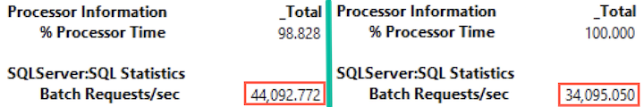
From performance standpoint, Standard Edition would suffice in many cases. Even though it lacks several nice features, it would work just fine even in large and busy systems. I dealt with many multi-TB installations that handled thousands transactions per second using Standard Edition of SQL Server.

Nevertheless, Standard edition lacks many of availability features offered in Enterprise Edition. Most important is index management. You cannot rebuild indexes keeping the table online. There are some tricks that can help reducing index rebuild time; however, it would not help much with the large tables.

This limitation has another interesting implication. In Standard Edition you cannot rebuild the indexes moving data to another filegroup transparently to the users. One of the cases when such an ability is very important is changing the database disk layout when you are upgrading disk subsystem. Obviously, it is very easy to do offline – this is just the matter of copying database files. However, even with the fast disk subsystem, that can take hours in multi-TB databases, which could violate your availability SLA.

This is especially critical with the Cloud installations where I/O subsystem is usually the biggest bottleneck due to the bad I/O performance. The situation, however, is starting to change. Both, Microsoft Azure and Amazon AWS now offer fast SSD-based I/O solutions for very reasonable price. Unfortunately, the old installations were usually deployed to the old and slow disks and upgrading to the new drives will often lead to the hours of the downtime.

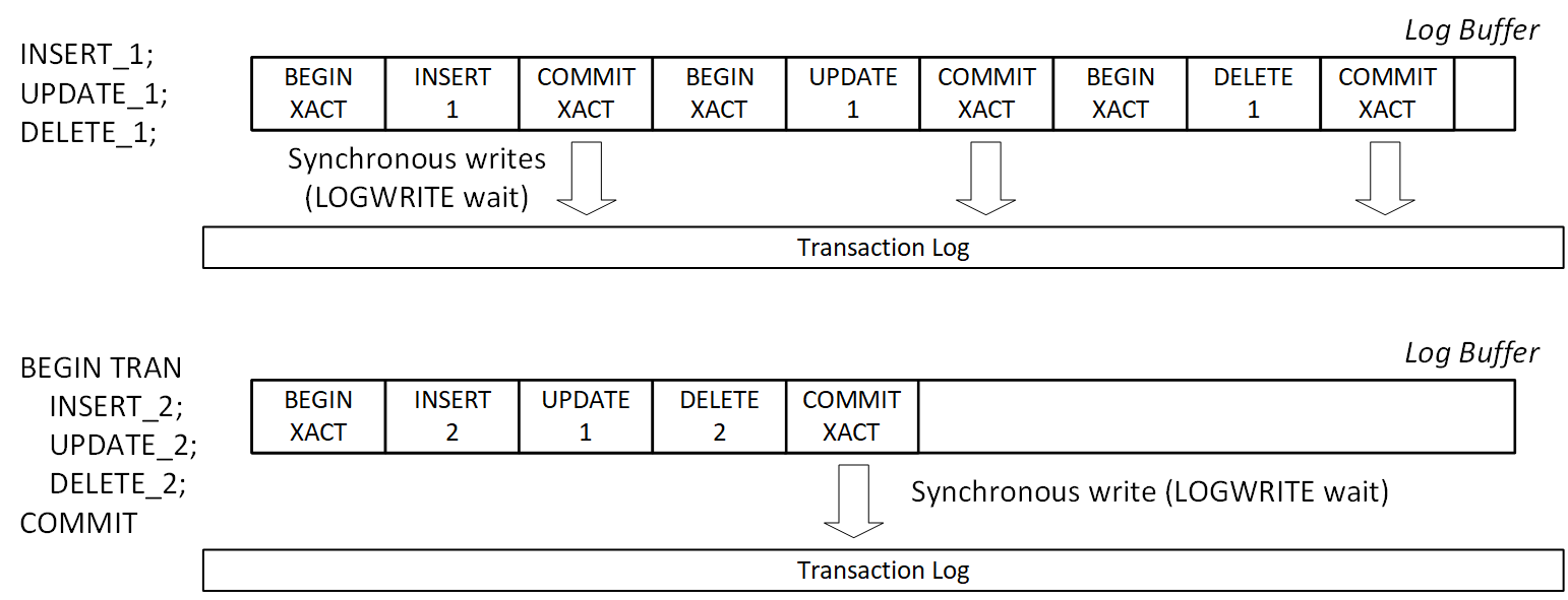
Fortunately, you can move data to the different disk arrays almost transparently to the users even in non-Enterprise Editions of SQL Servers. There are two ways how to accomplish it. The first one is very simple and can be done if system uses database mirroring. It requires failovers and secondary server downtime, which could lead to the data loss in case of disaster.

The second approach works without the mirroring. It is slow, it generates large amount of transaction log records, it introduces huge index fragmentation; however, it keeps database online most of the time. There is still the downtime involved; although, it could be limited to just a few minutes. It will work in any SQL Server version and edition – well, to be frank, I have not tried it in SQL Server 2000 yet.

Let’s look at both of those approaches in details.

Moving database files with mirroring Involved

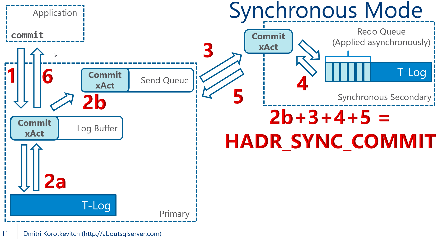
Database mirroring and, as matter of fact, Always On Availability Groups rely on the stream of transaction log records. Secondary servers apply the changes in the data files using file and page IDs as the reference. With exception of database file-related operations, for example file creation, primary and secondary servers do not need to store database files in the same location – it is possible to use different disk and folder structure on the servers.

You can rely on this behavior if you need to move database files to the different drives. You can run ALTER DATABASE MODIFY FILE(FILENAME=..) command on the secondary server, which will allow you to update data and log files paths in the system catalogs. Everything will continue run normally – those changes would not take place until the next database restart.

Unfortunately, you cannot take database that participate in the mirroring session offline and you need to shut down entire instance of SQL Server. After that, you can physically move database files to the new location. On the primary server, the database mirroring will switch to the DISCONNECTED state. The database will continue to be available to the clients; however, it remains unprotected – all changes will be lost in case of disaster. You need to remember that file copy operation can take hours and you need to evaluate if you can take such a risk. It is also worth to mention that transaction log on the primary would not truncate and continue to grow even after log backups – SQL Server needs to retain the log records until they sent to the secondary server.

After the file copy operation is completed, you can start the instance (the primary database will switch to SYNCHRONIZING state) and wait until all log records have been transmitted to the secondary (SYNCHRONIZED state). Then, you can failover and wash, rinse and repeat the process on the former primary server.

To summarize, this process is very simple and transparent to the client applications. It is the good choice as long as you can afford the instance downtime and possibility of  data loss in case of disaster. If this is not the case, you will have to use much more complicated approach.

When mirroring is not an option..

.. our life is much more complicated and the process will require multiple steps to complete.

1. We need to create the new data files in the secondary filegroups and shrink existing files by using DBCC SHRINKFILE(EMPTYFILE) command. This will move data from old to the new data files.
2. Next, we need to repeat the same process with the primary filegroup. You cannot remove primary MDF file from the database; although, you can make it very small and move all data from there.
3. Next, we need to shrink the transaction log .
4. Finally, we need to copy MDF and LDF files to the new location. This is offline operation; however, both, MDF and LDF data files are small at this point and downtime is minimal.

Let’s look at the process in details. As the first step, let’s create the test database with two filegroups and populate it with some data. For the demo purposes, I am assuming that C:\OldDrive folder represents old and C:\NewDrive – new disk arrays respectively.

create database DataMovementDemo
on primary
( name = N'DataMovementDemo', filename = N'C:\OldDrive\DataMovementDemo.mdf', size = 100MB, filegrowth = 50MB),
filegroup [Secondary]
( name = N'DataMovementDemo_Secondary1', filename = N'C:\OldDrive\DataMovementDemo_Secondary1.ndf', size = 100MB, filegrowth = 50MB),
( name = N'DataMovementDemo_Secondary2', filename = N'C:\OldDrive\DataMovementDemo_Secondary2.ndf', size = 100MB, filegrowth = 50MB)
log on
( name = N'DataMovementDemo_log', filename = N'C:\OldDrive\DataMovementDemo_log.ldf', size = 500MB, filegrowth = 500MB)
Go

alter database DataMovementDemo set recovery full
go

use DataMovementDemo
go

create table dbo.DataOnPrimary
(
    ID int not null,
    Placeholder char(8000),
    constraint PK_DataOnPrimary
    primary key clustered(ID)
    on [Primary]
);

create table dbo.DataOnSecondary
(
    ID int not null,
    Placeholder char(8000),
    constraint PK_DataOnSecondary
    primary key clustered(ID)
    on [Secondary]
);

;with N1(C) as (select 0 union all select 0) -- 2 rows
,N2(C) as (select 0 from N1 as T1 cross join N1 as T2) -- 4 rows
,N3(C) as (select 0 from N2 as T1 cross join N2 as T2) -- 16 rows
,N4(C) as (select 0 from N3 as T1 cross join N3 as T2) -- 256 rows
,N5(C) as (select 0 from N4 as T1 cross join N4 as T2 ) -- 65,536 rows
,Nums(Num) as (select row_number() over (order by (select null)) from N5)
    insert into dbo.DataOnPrimary(ID)
        select Num from Nums;

insert into dbo.DataOnSecondary(ID)
    select ID from dbo.DataOnPrimary;

We can check the size of the data and log files along with their free space with the code below.

select 
    f.name as [FileName]
    ,fg.name as [FileGroup]
    ,f.physical_name as [Path]
    ,f.size / 128.0 as [CurrentSizeMB]
    ,convert(int,fileproperty(f.name,'SpaceUsed')) / 
        128.0 as [UsedSpaceMB]
    ,f.size / 128.0 - convert(int,fileproperty(f.name,'SpaceUsed')) / 
        128.0 as [FreeSpaceMb]
from 
    sys.database_files f left join sys.filegroups fg on 
        f.data_space_id = fg.data_space_id;

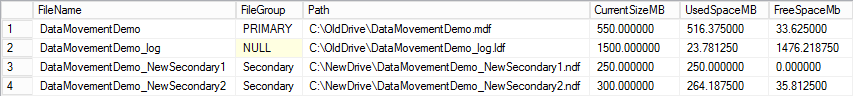
Figure 1 shows the output of the statement.

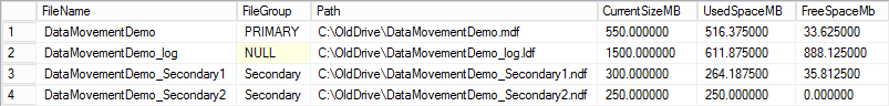
01. Database file stats after database creation

Moving data files from secondary filegroups

As the first step, you need to create new data files on the target drive. You can keep the same number of files as before, or use this as the opportunity to change the filegroup layout. In general, the number of files in the fielgroup greatly depends on the volatility of the data. Every data file has its own set of allocation map pages, which reduces the contention during page and extent allocations. It is impossible to give the general advice on how many files to create – I usually start with four files per filegroup unless the data is extremely volatile and the filegroup handles hundreds or even thousands of inserts per second. You can monitor and analyze PAGELATCH waits to see if there is the contention and adjust the number of the files accordingly.

In our example, let’s create two data files on C:\NewDrive folder as shown below. Make sure that both files have exactly the same initial size and autogrowth parameters specified in MB. This will help SQL Server to evenly distribute data between them.

alter database DataMovementDemo add file 
( name = N'DataMovementDemo_NewSecondary1', filename = N'C:\NewDrive\DataMovementDemo_NewSecondary1.ndf', size = 250MB, filegrowth = 50MB )
to filegroup [Secondary];

alter database DataMovementDemo add file 
( name = N'DataMovementDemo_NewSecondary2', filename = N'C:\NewDrive\DataMovementDemo_NewSecondary2.ndf', size = 250MB, filegrowth = 50MB )
to filegroup [Secondary];

Figure 2 shows the output from the Listing 2 after new files were created.

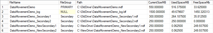
02. File stats after new files has been created

The DBCC SHIRINKFILE command works in a very simple manner. It reads allocated extents from the end of the file and moves them to the other files in the filegroup. In case, if  filegroup has multiple files, SQL Server uses proportional fill algorithm choosing to which file those extents need to be moved. The choice depends on amount of free space in the file – more space file has, more data would be copied there.

In case, when the filegroup originally has more than one file, you would like to avoid an overhead of moving data to the file, which yet to be moved. In our case, you want the data from DataMovementDemo_Secondary1 file to be distributed only between DataMovementDemo_NewSecondary1 and DataMovementDemo_NewSecondary2 files avoiding any inserts into DataMovementDemo_Secondary2 file.

Usually, data files in production databases do not have excessive amount of free space. When this is the case, you can simply prevent unnecessary data movements by restricting auto-growth of the old files. However, if those files have large amount of free space, you can also consider to shrink them and release this space first. There is the catch though. If free space is located in the beginning of the data file, shrink operation would start data movement and introduce the overhead. You need to make decision how to proceed on case by case basis.

The next listing shows how you can restrict the auto-growth for the file.

declare
    @MaxFileSizeMB int
    ,@SQL nvarchar(max)
	
-- Obtaining current file size 	
select @MaxFileSizeMB = size / 128 + 1
from sys.database_files
where name = 'DataMovementDemo_Secondary2';

set @SQL = N'alter database DataMovementDemo 
modify file(name=N''DataMovementDemo_Secondary2'',maxsize=' + 
    convert(nvarchar(32),@MaxFileSizeMB) + N'MB);';

exec sp_executesql @SQL;

Now we are ready to process the first data file. Listing below shows the code that performs data movement and removes an empty file from the filegroup afterwards. Both operations are transparent to the users and client applications. It is worth mentioning that you can use the code from the second listing above to monitor the progress of the operation. You can also look at percent_complete column in sys.dm_exec_requests view.

dbcc shrinkfile(DataMovementDemo_Secondary1, emptyfile);
alter database DataMovementDemo remove file DataMovementDemo_Secondary1;

If you checked the status of the files after operation is completed, you would see the results as shown in Figure 3. As you see, the data from the data file has been distributed between other files in the filegroup.

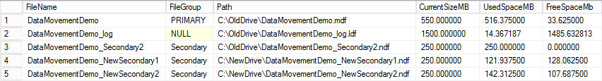
03. File stats after the first file has been processed

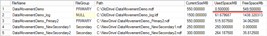
You can use exactly the same approach to move data from the DataMovementDemo_Secondary2 file. Listing shows the code and Figure 4 shows the database files after the process is completed. As you see, the secondary filegroup now resides on the new drive.

dbcc shrinkfile(DataMovementDemo_Secondary2, emptyfile);
alter database DataMovementDemo remove file DataMovementDemo_Secondary2;

04. File stats after the second file movement

The word of caution. As I already mentioned, DBCC SHRINKFILE  generates enormous amount of transaction log records. Make sure that transaction log is truncating especially if the database uses FULL recovery model.

Moving primary data file

Even though many of us know about the best practice of keeping PRIMARY filegroup empty, it rarely followed. Majority of production databases keep the data in PRIMARY filegroup, which usually consist of the single MDF file.

Unfortunately, you cannot remove nor change the primary data file in the database. Moreover, you cannot shrink the file below the size of the data currently stored in the file, even if a filegroup has the other data files.

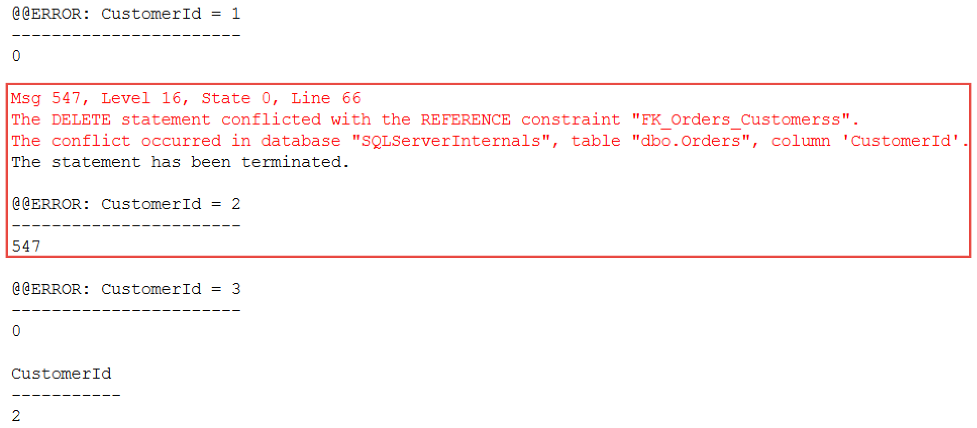
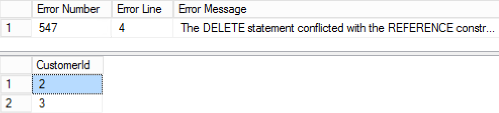
Fortunately, you can still use DBCC SHRINKFILE(EMPTYFILE) command on MDF data file. It would move data to the other files in the filegroup and failing on the final stage of the execution with the error message shown in Figure 5. Nevertheless, the majority of the data from the MDF data file would be moved to the other files.

05. DBCC SHRINKFILE(EMPTYFILE) error on the primary data file

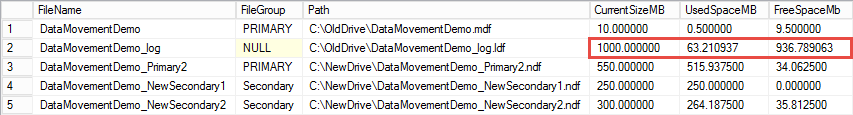
Listing below shows the code that performs this action. It creates the second data file in PRIMARY filegroup and moves the data from MDF file there. Figure 6 shows the file stats after it is completed – after DBCC SHRINKFILE(EMPTYFILE) error.

alter database DataMovementDemo add file 
( name = N'DataMovementDemo_Primary2', filename = N'C:\NewDrive\DataMovementDemo_Primary2.ndf', size = 550MB, filegrowth = 50MB )
to filegroup [Primary];
go

-- It will error in the end
dbcc shrinkfile(DataMovementDemo, emptyfile);

06.File stats after DBCC SHRINKFILE(EMPTYFILE) error

As you see, MDF data file is pretty much empty. You can release the empty space from the file using DBCC SHRINKFILE(DataMovementDemo, 10) command. Figure 7 illustrates the situation after it is completed and MDF file became very small.

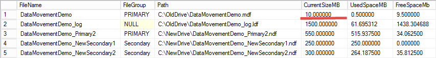
07. File stats after removal free space from MDF file

Unfortunately, this approach introduces two or more unevenly sized data files in the PRIMARY filegroup, which makes proportional fill algorithm less efficient. It may or may not be a problem in your system, depending on how volatile is the data. You can address it after you move MDF file to the new drive by creating other data files in PRIMARY filegroup and shrinking and emptying the file you just created. This will distribute the data in all files in the filegroup evenly.

Finally, it is worth mentioning that in some cases, especially when MDF file is very large, DBCC SHRINKFILE(EMPTYFILE) command can error in the middle of the execution stating that it cannot move some of the data pages that belong to the system objects. You can address it by re-running DBCC SHRINKFILE using the current data size as the target (e.g. releasing the empty space from the file). This will move those data pages within the file and you can re-run DBCC SHRINKFILE(EMPTYFILE) command afterwards.

Shrinking transaction log

The decision how to handle transaction log depends on its size, and backup and high availability strategies you have in place. Transaction log size affects time, which file copy operation will require and, therefore, the system downtime. Obviously, the simplest solution is avoid shrinking transaction log if the log file is not very large and downtime is acceptable.

In case, if you need to reduce the downtime, there are no options but shrinking the log file. It is usually not a problem in case if database uses the SIMPLE recovery model. However, with FULL recovery model situation is a bit more complicated.

As the first step in this process, you need to truncate the log by performing the log backup. This operation does not decrease the size of the log file but rather reduce the size of the active/used portion of the log. Keep in mind that open transactions, backlogs in high availability log record queues and a few others factors can prevent transaction log from being truncated.

Next, you can shrink the log file using DBCC SHRINKFILE command with the very small size- 50MB, for example- as the target. Your results may vary. Internally, SQL Server splits the log to the multiple blocks called Virtual Log Files and re-uses them in the circular matter. Shrink operation would release the empty space from the tail of the log; however, the resulting file size depends on the active VLF offsets in the file.  It is entirely possible that shrink command would not reduce the file size if active VLFs are close to the end of the file.

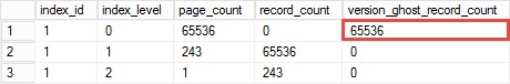
Let’s illustrate that with the example and run DBCC LOGINFO command, which shows the status of the VLFs in the log file. Figure 8 illustrates the partial output from our test database. Status value of 2 indicates that VLF is active and cannot be truncated. As you can see, it is in the middle of the file.

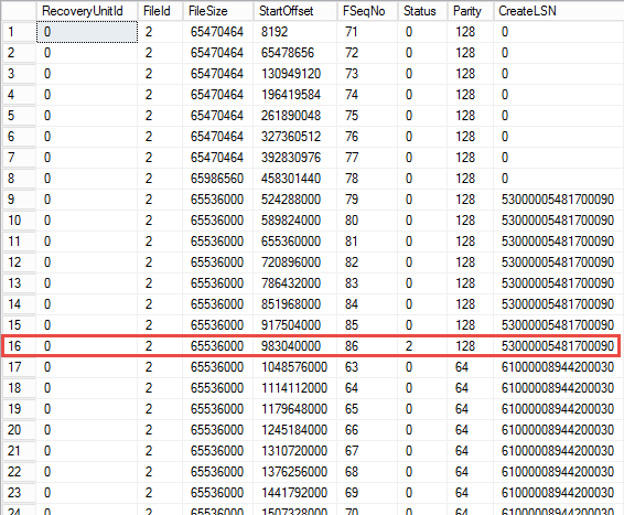
08. DBCC LOGINFO output

As you saw in Figure 7, the log file is using just 61MB out of 1.5GB in the file. However, if you run DBCC SHRINKFILE(DataMovementDemo_Log, 65) command, you’d see that it did not shrink beyond 1000MB as shown in Figure 9.

09. File stats after shrinking transaction log

If you run DBCC LOGINFO again, you would see that SQL Server removed the empty VLFs from the end of the file and stopped when it reached the active VLF there. Figure 10 illustrates that. It is also worth mentioning that the first VLF in the file also became active during the shrink.

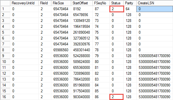
10. DBCC LOGINFO output after shrinking transaction log

At this point you have the two options, assuming that size of the log file is still unacceptable. You can wait until SQL Server truncates the log making last VLF inactive and repeat the shrink operation afterwards. This will eventually happen with the regular workflow. You can even force this by generating transaction log records by creating the table with one CHAR(8000) column and inserting multiple rows there in the separate transactions and batches. Do not forget to force log truncation with BACKUP LOG operations and use DBCC LOGINFO to monitor the progress.

Alternative option is switching database to the SIMPLE recovery model using ALTER DATABASE SET RECOVERY SIMPLE command. This will perform log truncation and will allow you to shrink the log to the minimal size immediately. Obviously, this approach will require you to disable transaction log-based high availability technologies and recreate backup chain afterwards.

While, on the surface, switching database to SIMPLE recovery model introduces unnecessary complications, it could be the good opportunity to rebuild transaction log file. Large number of VLFs negatively affect system performance and can slow down database recovery time. Unfortunately, default settings in New Database dialog in Management Studio leads to that situation. At least in SQL Server prior 2016.

You can rebuild transaction log after you moved the file to the new drive by manually growing it in 4000MB chunks – do not use 4GB chunks due to the bug in some of SQL Server versions. Every chunk will generate 16 250MB VLF files, which works well for the most configurations.  After that, change log auto-growth to be in MB – I found that 1000MB chunks are good for majority of the cases.

Moving MDF and LOG files to the new drive

Finally, it is the time to move MDF and LDF files to the new drive. Unfortunately, it is offline operation. Fortunately, at this point, both files should be very small and downtime should be minimal.

As the first step, you need to change location of the files using ALTER DATABASE MODIFY FILE command. This will change location of the files in the system catalogs, and will take an effect after the database restart.

Next, you can take database offline using ALTER DATABASE .. SET OFFLINE WITH ROLLBACK IMMEDIATE command. This will disconnect all users from the database rolling back the active transactions. You can copy the files and take database back online using ALTER DATABASE .. SET ONLINE command as shown below.

use master
go

alter database DataMovementDemo modify file
( name = N'DataMovementDemo', filename = N'C:\NewDrive\DataMovementDemo.mdf');
alter database DataMovementDemo modify file
( name = N'DataMovementDemo_Log', filename = N'C:\NewDrive\DataMovementDemo_Log.ldf');
go

alter database DataMovementDemo set offline with rollback immediate
go

-- COPY FILES 

alter database DataMovementDemo set online;

As you see in Figure 11 – our database is now residing on the new drive.

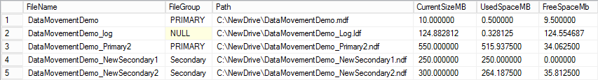
11. Final file layout

Almost done! Again, do not forget to rebuild the log file and switch database to FULL recovery model if needed.

Dealing with index fragmentation

There is one final step though. As you already know, DBCC SHRINKFILE command works on the extent level. It moves allocated extents from the end of the file to the new place without any considerations to which objects those extents belong. As you can guess, this leads to the huge index fragmentation, which you need to address at the final stage of the process.

Obviously, you do not want to acquire Schema Modification (SCH-M) locks blocking access to the tables during index rebuild operations. It makes index reorg the better choice for this scenario – it is online in any edition of SQL Server.

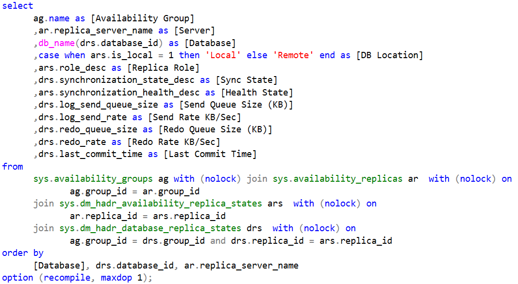
Listing below shows the script you can use to generate ALTER INDEX REORG commands for every clustered and nonclustered indexes from specific filegroup. It returns result as XML string – you can simply cut and paste it and run as another batch.

;with FGObjects(SchemaName, TableName, IndexName, RowNum, Cnt)
as
(
    select 
        s.Name, t.Name, i.Name
        ,ROW_NUMBER() over(order by t.object_id, i.index_id) as RowNum
        ,COUNT(*) over() as Cnt
    from
        sys.indexes i join sys.filegroups f on
            i.data_space_id = f.data_space_id
        join sys.all_objects t on
            i.object_id = t.object_id
        join sys.schemas s on
            t.schema_id = s.schema_id
    where
        i.index_id >= 1 and
        t.type = 'U' and -- User Created Tables
        i.data_space_id = f.data_space_id and
        f.name = 'PRIMARY' -- Filegroup
)
select 
    'alter index ' as [text()]
    ,[IndexName] as [text()]
    ,' on ' + SchemaName + '.' as [text()]
    ,[TableName] as [text()]
    ,' reorganize;' + CHAR(13) + CHAR(10) as [text()]
    ,'raiserror(''' as [text()]
    ,RowNum as [text()]
    ,'/' as [text()]
    ,Cnt as [text()]
    ,' is done'',0,1) with nowait;' + CHAR(13) + CHAR(10) as [text()]
    ,'go' + CHAR(13) + CHAR(10) as [text()]
from FGObjects
for xml path('');

As you see, the process of moving database files between different drives could lead to significant amount of work if you want to minimize the downtime. However, it is often the only choice, especially in the Cloud environment where you can get significant performance benefits by utilizing new SSD-based drives. Go for it! 🙂

Source code is available for download.