Category Archives: T-SQL

Locking in Microsoft SQL Server (Part 17) – Implementing Critical Section / Mutexes in T-SQL

Today I’d like us to discuss how we can implement analog of Critical Section (or Mutex) in T-SQL. One of the tasks when it could be beneficial is when we need to prevent the multiple sessions from reading the data simultaneously. As the example let’s think about the system which collects some data and does some kind of post processing after data is inserted.

One of the typical implementation in such architecture would be having the farm of the application servers that do the post processing. We usually need to have more than one server in such scenario for scalability and redundancy reasons. The key problem here is how to prevent the different servers from reading and processing the same data simultaneously. There are a few ways how we can do it. One approach would be using central management server that loads and distributes the data across processing servers. While it could help with the scalability we will need to do something to make that server redundant. Alternatively we can use some sort of distributed cache solution. We could load the data there and every server grabs and processes the data from the cache. That approach could be scalable and work great although distributed cache is not the easy thing to implement. There are the few (expensive) solutions on the market though if you don’t mind to spend money.

There are of course, other possibilities but perhaps the easiest approach from the coding standpoint would be implementing application servers in the stateless manner and do the serialization while reading the data in T-SQL.

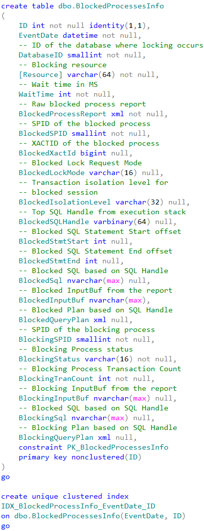
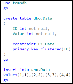
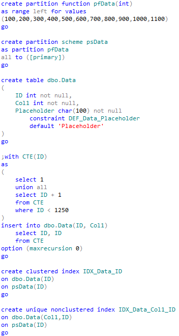
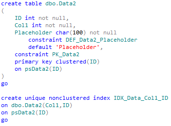
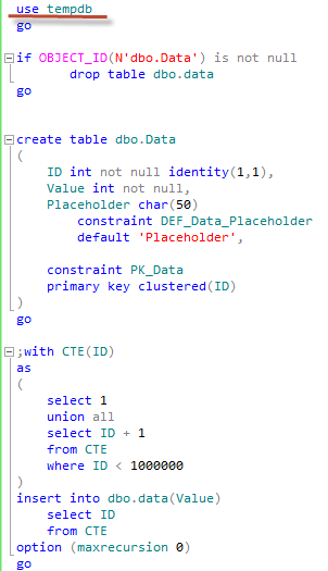
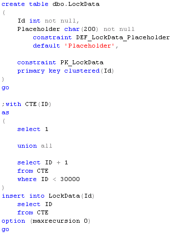
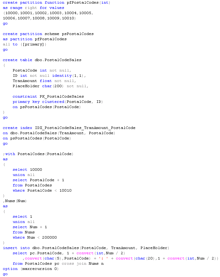
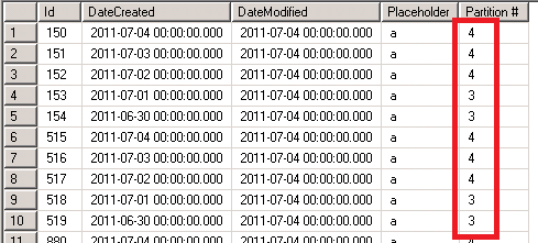
Let’s create the table we can use in our exercises and populate it with some data.

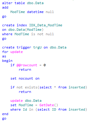
A couple things here. First of all, we need to handle the situations when application server crashes and make sure that data would be loaded again after some time by another app server. This is a reason why we are using ReadForProcessing datetime column rather than the simple Boolean flag.

I’d also assume that system wants to read data in FIFO (first in, first out) order as much as possible and after processing is done the data would be moved into another table and deleted from the original RawData table. This is the reason why there is no indexes but clustered primary key. If we need to keep the data in the same table we can do it with additional Boolean flag, for example Processed bit column, although we will need to have another index. Perhaps:

create nonclustered index IDX_RawData_ReadForProcessing
on dbo.RawData(ReadForProcessing)
include(Processed)
where Processed = 0

In addition to the index we also need to assign default value to ReadForProcessing column to avoid ISNULL predicate in the where clause to make it SARGable. We can use some value from the past. 2001-01-01 would work just fine.

In either case, after we read the data for the processing we need to update ReadyForProcessing column with the current (UTC) time. The code itself could look like that:

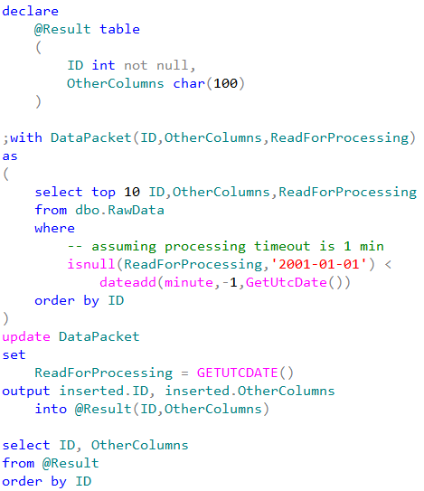
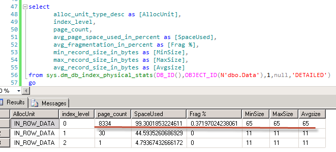
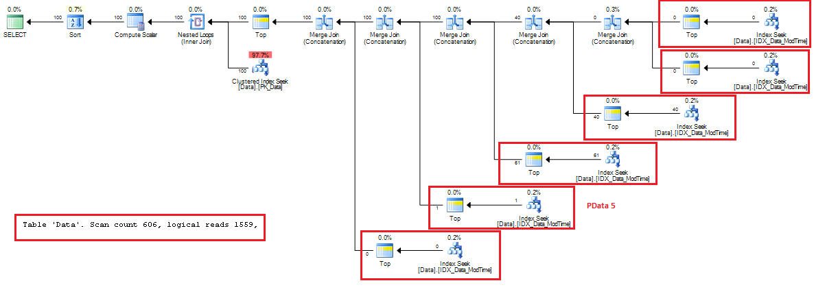
DataPacket CTE is using ordered clustered index scan. It would stop scanning immediately after read 10 rows (TOP condition). Again, we are assuming that data is moved to another table after the processing so it would be efficient. We are updating the timestamp same time when we read it and saving the package for the client in the temporary table @Result using output clause

The problem here is the race condition when two or more sessions are starting to read and update the data simultaneously. Our update statement would obtain shared (S) locks during select in CTE and after that use update (U) and exclusive (X) locks on the data to be updated.

Obviously different sessions would not be able to update the same rows simultaneously – one session will hold exclusive (X) lock on the row while other sessions would be blocked waiting for shared (S) or update (U) lock. In the first case (shared (S) lock), it’s not a problem – the blocked session will read new (updated) value of ReadForProcessing column as soon as the first session releases the exclusive (X) lock. But in the second case the second session will update (and read) the row the second time. Simplified version of the process is shown below.

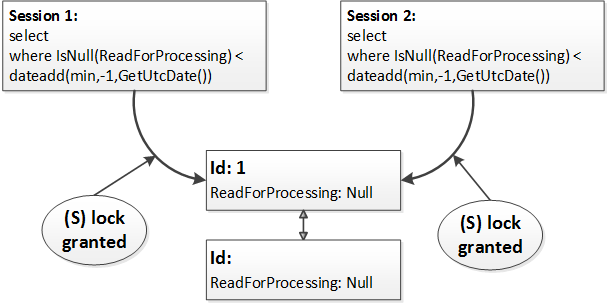
At the first step both sessions read the row acquiring and releasing shared (S) locks. Both sessions evaluate the predicate (isnull(ReadForProcessing,’2001-01-01′) < dateadd(minute,-1,GetUtcDate())) and decided to update the row. At this point one of the sessions acquires update(U) and then exclusive (X) lock while other session is blocked.

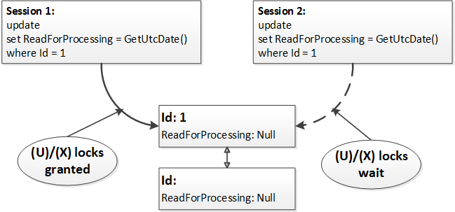
After the first session releases the exclusive (X) lock, the second session updates the same row.

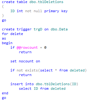
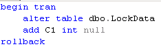
How can we avoid that? We can create another resource and acquire exclusive lock on that resource before update statement from within the transaction. As we remember, exclusive (X) locks held till the end of transaction, so we will use it as the serialization point. Let’s take a look how it works by creating another table as the lock resource. Now, if we start transaction, we can obtain exclusive table lock. Again, exclusive (X) locks held till the end of transaction, so other sessions would be blocked trying to acquire the lock on the table. As result, execution of our update statement would be serialized.

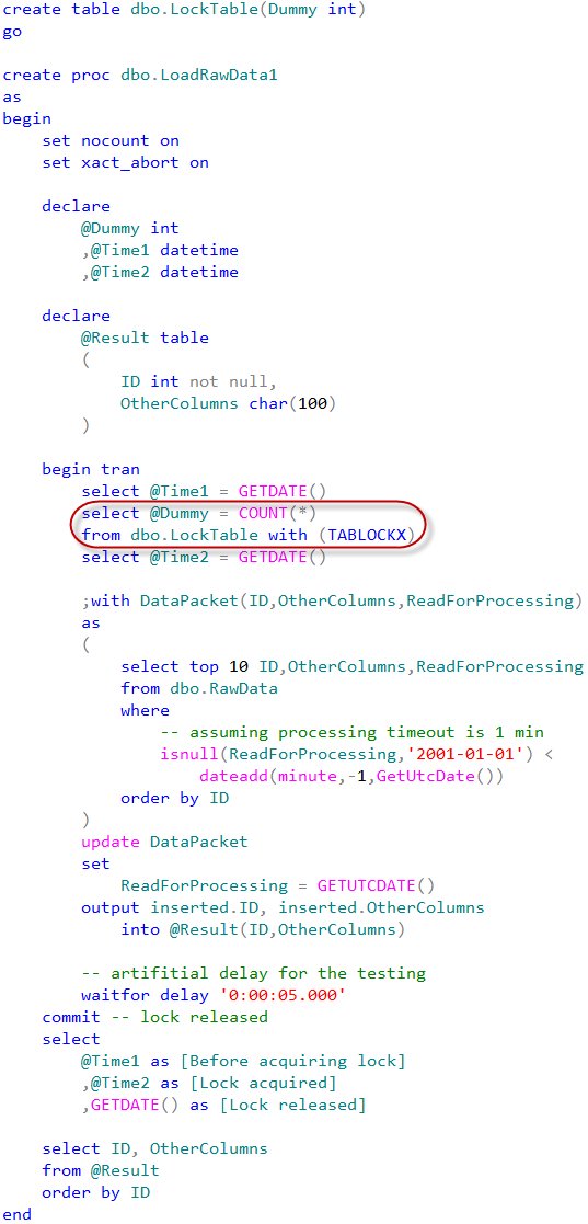
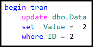
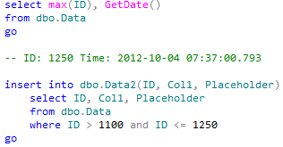
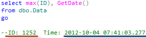
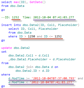
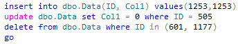
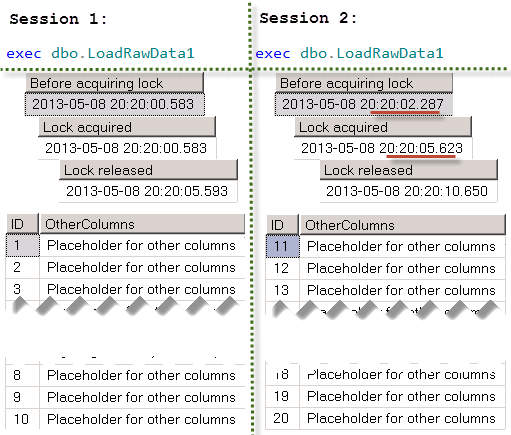
We can test that approach by running this SP from the multiple sessions simultaneously. There is the artificial delay which we are using during the testing just to make sure that we have enough time to run SP in the different session.

While that approach works, there is another, better way to accomplish the same task. We can use application locks. Basically, application locks are just the “named” locks we can issue. We can use them instead of locking table.

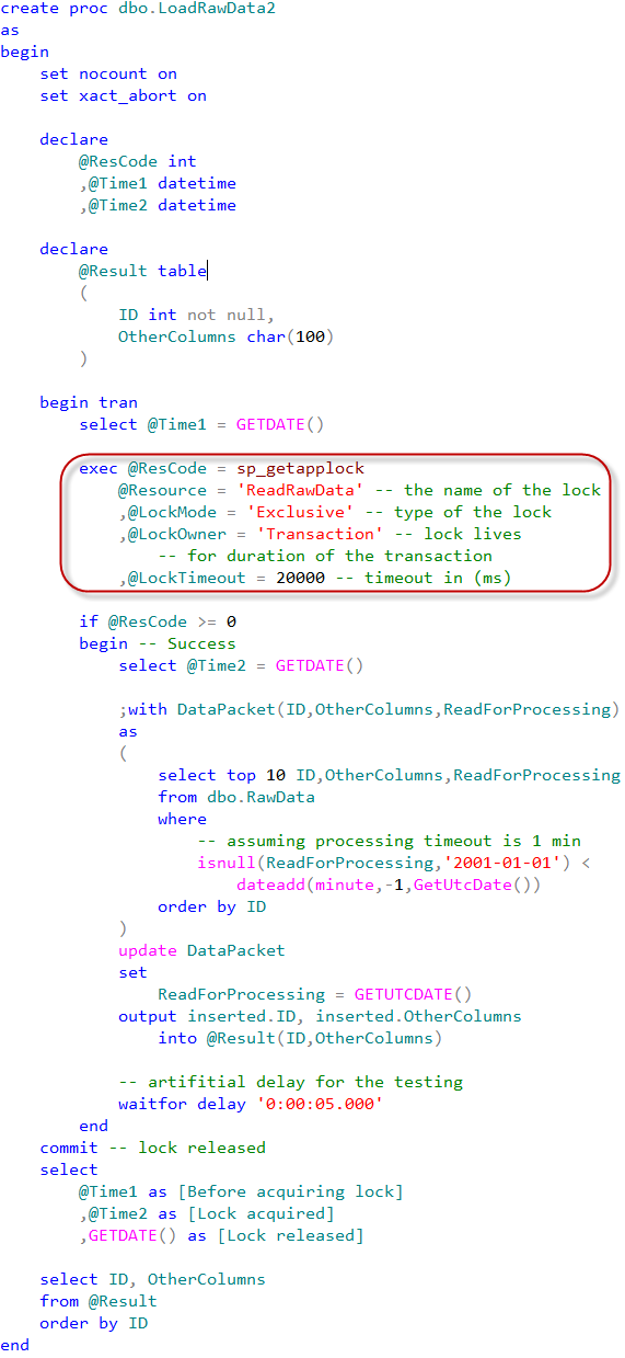
That would lead to the same results.

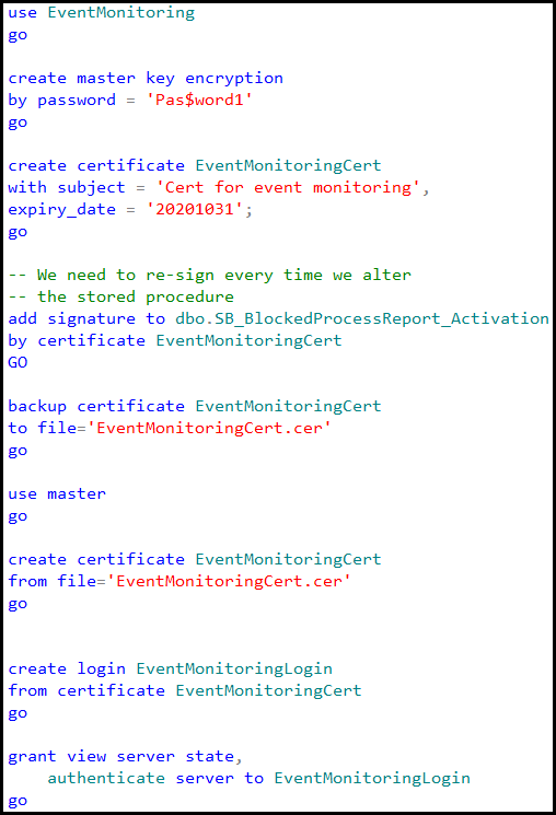
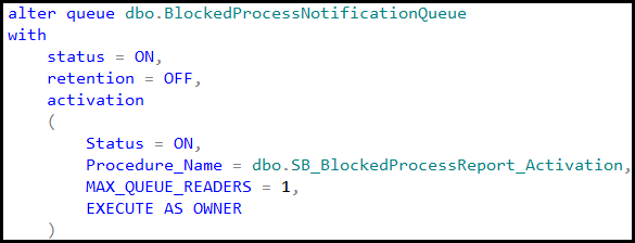
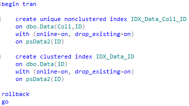
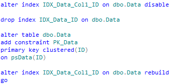
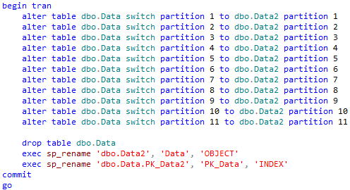
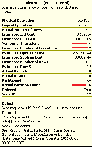
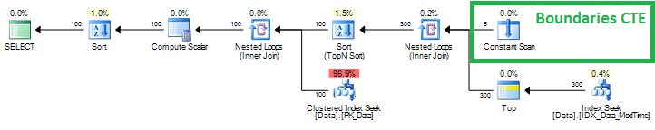
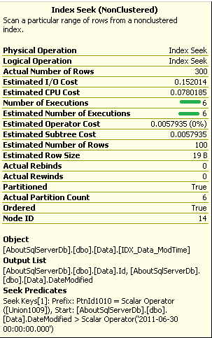
Application locks are also very useful when we need to implement some code that alters the database schema (for example alter partition function) in the systems that are running under load all the time (24×7). Our DDL statements can issue shared application locks while DDL statements acquire exclusive application locks. This would help to avoid deadlocks related to the lock partitioning. You can see the post about lock partitioning with more details about the problem and implementation.

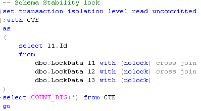
Although, if we talk about specific task of serialization of the reading process, we don’t need critical section at all. We can use the locking hints instead.

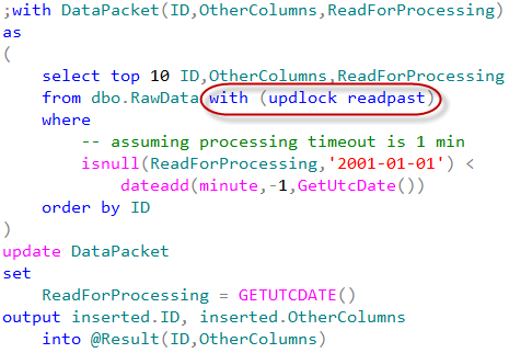
As you can see, there are two locking hints in the select statement. UPDLOCK hint forces SQL Server using update (U) locks rather than shared (S) ones. Update locks are incompatible with each other so multiple sessions would not be able to read the same row. Another hint – READPAST – tells SQL Server to skip the locked rows rather than being blocked. Let’s modify our stored procedure to use that approach.

I’m adding some code to the procedure to emulate race condition. In one session we will run the stored procedure with @UseDelay = 1. In another with @UseDelay = 0. Both of those sessions will start to execute the main update statement roughly at the same time.

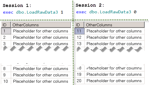
This method works even more efficiently than the “critical section” approach. Multiple sessions can read the data in parallel.

Well, I hope that we achieved two goals today. First – we learned how to implement critical section and/or mutexes in T-SQL. But, more importantly, I hope that it taught us that in some cases, the “classic” approach is not the best and we need to think out of the box. Even when this thinking involved the standard functional available in SQL Server.

Source code is available for download

Table of content

Next: Key lookup deadlock


Locking in Microsoft SQL Server (Part 16) – Monitoring Blocked Processes Report with Event Notifications

UPDATE 2018-08-01: New and redesigned version of the code is available here

As we already know it’s very easy to capture blocked process report by using SQL Traces. That method though has a few limitations. First of all, it means we need to have SQL Trace up and running all the time. And SQL Trace, especially the client one, introduces the overhead on SQL Server. Another big problem is that we need to monitor traces on the regular basis. And in case if we had the blocking from within the stored procedures (e.g. session input buffer contains SP reference only), we would need to use sql handles and get the estimate execution plan from the plan cache. Nothing guarantees that plan would be there by the time when we start troubleshooting the blocking problem. Of course, we can set up an alert with SQL Agent and get the notification when blocking
occurs although it would still mean that we have to do our job manually.

As another option we can use Event Notification for BLOCKED_PROCESS_REPORT event. This approach would utilize Service Broker so we would be able to create activation stored procedure and parse blocking report there. Let’s take a look at that.

First of all, we need to decide where to store the data. While we can put the table to the user database, I’d prefer to use separate utility database for the data collection. Let’s do that:

At that point we would have blocked process report events going to dbo.BlockedProcessNotificationQueue service broker queue. Assuming, of course, that we have blocked process threshold option set.

Obviously we do not want to have those messages sitting in the queue – it’s kind of defeating the purpose of having the process automated. What I would like to do at this point is shredding event data and putting it to the table for analysis. Another important factor is that blocked process monitor would generate separate events for the same blocking condition every time it wakes up. For example, if we have blocking process threshold set to 5 seconds, we can get five events until our query times out after 30 seconds. Ideally I’d like to combine those events into the single one to have analysis simplified. So let’s create the table to store the data.

This table stores the information about both – blocked and blocking processes. Although blocking information can be misleading in case if blocking session currently executes the different batch or even waiting for the next batch to be executed – table would store the current state rather than info at the time when blocking occurs. In any cases, from the blocking process standpoint the most interesting attributes are:

  1. Process Status – is it running, sleeping or suspended? If it’s sleeping, it could be the sign that client does not work with transations correctly – either did not commit one of the nested transactions or, perhaps, mixed them with UI activity. Suspended status could be the sign of the blocking chain which is another story
  2. TranCount – if it’s more than one, it would tell us that we have nested transactions and again, perhaps, client does not handle them correctly.

In any case, we will have full report stored and can access it if needed. And of course, we can modify the table and add extra attributes if we want to.

Now it’s the time to put the activation procedure in place. I’m going to cheat a little bit here – click at the link to the source code at the end of the post to see it.

There are two things I’d like to mention though. First one is how we get the query plans.  For the blocked process we are trying to get it from sys.dm_exec_requests first. This is the only bullet-proof way to get the real plan but it would work only if the statement is still blocked when activation SP executes. If this is not the case we are using sys.dm_exec_query_stats DMV. There are a couple challenges though. First, there is the chance that plan would not be there – for example in case of the memory pressure. Alternatively we have the situation when there are multiple plans due recompilation. We are trying to guess the right one by filtering based on the blocking time but that method is not always working. So no guarantees. For the blocking process we are always using sys.dm_exec_query_stats picking up the top (random) plan.

Another thing is how we are looking up if there are other events for the same blocking. Basically stored procedure is trying to match various columns in the merge statement – perhaps even more than needed – but in either case I’d rather have duplicate records than incorrect information.

Last step we need to do is setting up the security. That step is kind of optional in case if we are storing the data in the user database but in our case, when we create the blank database and set up everything under “dbo” user it’s required. When Service Broker activates the stored procedure under that security context (EXECUTE AS OWNER), dbo has enough rights to deal with the database object. But that user also needs to have the rights to query system DMV. As result, we need to create the certificate in the both, EventMonitoring and master databases, create the login from the certificate, grant this login “view server state” and “authenticate server” rights and finally sign the stored procedure with the certificate. Or, perhaps, mark the database as Trustworthy 🙂

And now it’s time for the testing. Let’s create the small table and populate it with a few records.

Next, let’s place exclusive (X) lock on one of the rows in the first session.

In another session let’s introduce the table scan in read committed isolation level.

If we query the service broker queue we would see that there are a few events there. Our queue does not have automatic activation yet.

And finally let’s alter the queue to enable the activation.

Next, let’s query the table.

As we can see, there is the single record in the table now – exactly what we need. This approach is, of course, customizable. You can collect other statistics by changing the implementation. Hope, that script would be the great starting point

Next: Implementing Critical Sections / Mutexes in T-SQL

Table of content


Sliding window scenario – when data spilled out to the right-most partition

After my last post I’ve received a couple emails asking how did I fix the problem. Just to remind – data spilled out to the right-most partition of the table and as result sliding window scenario did not work anymore. When process tried to split right-most, non-empty partition, it obtained long-time schema modification (SCH-M) lock. And then start to scan/move data while all access to the table was blocked. Today we are going to discuss how to fix that.

The most important question is if we can put the system offline during that operation. If this is not the case, well, our life becomes much more complicated. And our options for online recovery are rather limited. Let’s take a look. First, I would create partition function, scheme, table and populate it with some data with ID between 1 and 1250.

As you can see, I duplicated the case we had – we spilled out some data to the right most partition (with ID > 1100) which should be empty.

Let’s create another correct partition function and scheme:

For online recovery we can re-create our indexes online moving them to another partition. I’m doing it as part of transaction just to roll everything back to the initial “invalid” stage.

This operation would run with the minimal locking and achieve our goal. There are 3 things worth to mention though. First – online index rebuild uses row versioning and as result you will introduce quite heavy tempdb usage during that operation. Next, we are “rebuilding” much more data than actually needed – think about it – we have just one (right most) partition that needs to be recreated but we are rebuilding entire table. But more critical for us that this approach would not work if you have primary key constraint defined on the table. Unfortunately there is no way to recreate constraint moving it to another partition. Basically it means that you would not be able to resolve the issue without putting your system offline. Well, to be exact, if you have non-clustered primary key you can replace it with unique non-clustered index if this is acceptable. But still..

So what can we do with the primary key constraint? First, let’s prepare our table. As the side note – I’m disabling non-clustered index to prevent extra rebuild when we drop the clustered index.

As I mentioned before, we would not be able to do the operation without putting system offline. The goal though is to reduce offline time as well as to process/move as little data as possible (our right most partition only).

First of all, let’s create another table with indexes using new (corrected) partition scheme.

The problem here is that new table should have exactly the same physical row structure with the old one. And if you dropped or altered any column in the old table, your physical structure would not match table definition. If this is the case, you’ll need to create and alter the new table in the same way. Simplest way to compare is to run the following statement after new table is created.


I strongly suggest to test that you did not miss anything with the latest backup. Otherwise you could end up in the nasty situation when your data spread across multiple tables.

Anyway, assuming everything is fine our action plan would be:

  1. Copy all data from invalid partition(s) from Data to Data2. Let’s say that step starts at time T1.
  2. Apply all data changes that happened between T1 and now. Assuming that step starts at time T2. This step is optional but it would reduce downtime
  3. Put system offline
  4. Apply all changes from Data that happened between T2 and now. No new changes would be done in Data during this step because system is offline
  5. Switch all “normal” partitions from Data to Data2
  6. At this point Data would have only right-most incorrect partition, Drop (or rename) the table.
  7. Rename Data2 to Data (including constraints)
  8. Bring system online

Obviously one of the questions is how to find what is changing in the table while we are running steps 1 and 2. Well, it depends, of course. If you have identity or sequence keys, you can use them to track inserts. For updates – you can log time of update – perhaps by creating the new column and populating it with the trigger. For deletions – trigger again. Let’s do our prep work. I assume in that example that we are using sequences (or identity) for inserts. First – updates.

Now deletions. I’m using very simple approach here and going to apply all deletions at once during step 4.

Now we are ready to go. At the beginning of the step 1 we will log our ID and time to use it later.

This step would be quite time consuming and depend on amount of data we are copying. I’m also going to emulate some update activity in Data.

Now we need to apply changes in the original table that were made during step 1. Generally speaking, we can skip this step because we are going to do that again later when system is offline. But remember – our system is still online and this step would reduce downtime. In fact, if you have heavy activity you’d probably like to run this step again a few times.

As I mentioned before – I’m going to cut a corner here and don’t deal with deletions during that step. Again, we need to log ID and current time at the beginning of this step.

Again, I’m emulating some update activity in the system

Now it’s time to put system offline. And if your system is truly offline at this point, it’s also the good idea to create database snapshot to be able to “rollback” the changes.

So let’s apply all updates again including deletion activity.

Now we are almost ready to switch partitions. Only thing we need to do before is dropping our ModTime column and index we created.

And now the key part – switch and rename.

Now we can bring the system online and do the final clean up.

As you can see, the process is a bit complex. But at the end it minimizes the downtime. One thing to keep in mind – partition scheme and functions have been recreated under the new name so you need to take care of the code that references the old ones. SQL Search is your friend here.

While problem is fixed now the best way to deal with such kind of problems is don’t have them at all. As I mentioned before – all of that could be avoided if the size of partition has been re-evaluated from time to time.

The source code is available for download

Cautionary tale about triggers, version store and fragmentation

A while ago triggers were slow. Very slow. In the versions prior to SQL Server 2005, triggers scanned transaction log in order to build internal inserted and deleted tables. That approach has been changed in SQL Server 2005 when triggers started to use version store – similarly to what optimistic locking is using. That helps with performance but same time introduces a few interesting issues. Let’s take a look.

First of all, let’s create a table and populate it with some data. I would like to point that I’m using tempdb in that example mainly to show that this behavior is completely independent from transaction isolation levels and optimistic locking database options.

Now let’s take a look at what we have in the index (click on the image to open it in the different tab)

As you can see, we have 65 bytes rows without any fragmentation. So far so good. Now let’s update Value column.

We updated fixed-width column. Row size has not changed. No fragmentation here. As the next step let’s create a trigger.

As you see, trigger itself is empty – we don’t even access inserted/deleted tables there. Now let’s update our table again

Still the same thing. But if we look at performance monitor counters – we can see that update now generates version store activity.

As the next step I’d like to add LOB column to the table. I’m using varchar(max) but you can replace it with nvarchar, binary, xml or clr data type. It would be the same.


Column is nullable so alteration here is pure metadata operation. And now let’s run the update statement.

Oops – now we have 14 bytes version store pointer added to the row. That introduces heavy fragmentation (new versions are larger so they don’t fit into the pages) and double our storage space. Well, a little bit unexpected development. Generally speaking this is very similar problem with what we have with data modifications when we use optimistic isolation levels.

OK, it happens with LOB columns. Now let’s check the case when ROW OVERFLOW is possible. Let’s drop LOB column and add to varchar(5000) columns here.


Again, we rebuilt the index – 14 bytes pointers are went away. Now let’s run update statement again.

Same thing – extra 14 bytes and fragmentation.

And let’s prove that trigger is the problem. First, let’s drop the trigger and rebuild the index

And next – run update again.

As you can there are no 14 bytes version store pointer nor fragmentation.

At last, let’s take a look at the very interesting thing – let’s see what happens when we have ON DELETE trigger. Generally speaking, when we delete the row, only thing that SQL Server initially does is mark row as the “ghost” row. Just the change in the header. But with the trigger the situation could be different.

You can see, that in our case we ended up with page split on delete!

This behavior adds extra arguments to the discussion why triggers are bad in general. Triggers add extra load to tempdb. And in case if you have the possibility of row overflow or LOB allocations, you’d end up with 14 bytes version store pointer and extra fragmentation.

Source code is available for download

P.S. I’d like to thank Paul White for his help with that post.

Locking in Microsoft SQL Server (Part 14) – Deadlocks during DDL operations (alteration, partition switch, etc)

Today I’d like us to talk about one practical problem related with the locking – how to deal with deadlocks during DDL operations. For example, table and partition functions alteration, partition switch and others. This problem is very common in OLTP environment when table is constantly querying by the multiple sessions. One of the common examples there is sliding window pattern when the table has been partitioned based on some time interval (daily, weekly, monthly, etc) and data has been purged on the regular basis by switching partition to the temporary table. Let’s try to understand why we have deadlocks here and what we can do to solve the problem.

First of all, as the pre-requirement, let’s assume that we implemented our partitioning correctly. Most important factor is that our operation does not require any data movement nor scans. For example, we don’t split ranges in partition function in the way that requires  physically move the data to another partition (e.g. we are pre-allocating empty partition rather than splitting the range with the value at the middle of the partition that has some data). In that case partition operations are purely metadata operations and only schema locks are involved.

Another thing to avoid is mixing DML and DDL statements in one transaction. Let’s think about following example (let’s ignore page locks and schema stability (SCH-S) locks for simplicity sake):

  1. Session 1 starts transaction and updates 1 row in the table. E.g. at this stage we will have (X) lock on the row and (IX) lock on the table
  2. Session 2 is trying to select data from the table and being blocked by Session 1. So now we have Session 2 waiting for (S) lock on the row and also have (IS) lock acquired on the table
  3. Now session 1 is trying to implement partition switch. For that operation (SCH-M) lock needs to be acquired on the table and it would be blocked by (IS) lock from the Session 2.

Classic deadlock. But let’s assume that this is not the case. What happens when we have multiple locks on the same object? Generally speaking, lock requests would be serialized. In some cases existing locks could be even re-used. Let’s see that. First, let’s create a table and add a few records there.  Next, let’s have session 1 to read one row in repeatable read mode. As we remember it would hold (S) lock on the resource. Again, for simplicity sake let’s look at the row (key) level locks only

Now let’s try to update the row in another session. This session will try to acquire (X) lock on the resource and would be blocked because (X) lock is not compatible with (S) lock.

Now let’s try to read the same row in read committed mode from the 3rd session. As we can see everything works without blocking.

Let’s try to look at what locks were acquired using SQL Profiler.

As you see session acquired intent (IS) locks but did not acquire shared (S) lock. There is (S) lock from the session 1 already which guarantees that row has not been modified by uncommitted transactions. No reasons to acquire another (S) lock because in read committed isolation level (S) locks on the rows have been released immediately.

But what will happen if we try to read the row in repeatable read mode again? In that isolation level session needs to keep the (S) lock until end of transaction and it’s a reason why it’s trying to acquire the lock.

As you can see – it’s being blocked because there is (X) lock in the queue. So in order to be granted lock needs to be compatible with the all locks on that resource – does not matter granted or now.

It’s worth to mention that the first scenario, when session 3 ran in read committed mode and did not acquire the lock on the resource, can be considered as internal optimization. In some cases SQL Server still acquires another shared (S) lock there even if there is another shared (S) lock held. In such case the query would be blocked similarly to repeatable read transaction isolation level.

Keeping all this in mind we can ask – why would we have deadlocks if locks are serialized? Would not the session with schema modification (sch-m) lock wait till other locks are released and proceed from there? Yes and no. Let’s put one other thing to the mix – lock partitioning. This is quite confusing term and does not have anything to do with table partitioning. In nutshells when server has 16 or more CPUs (think about dual quad-core with hyperthreading enabled) SQL Server starts to partition intent (IS, IX, IU) and schema stability (SCH-S) object locks on per-cpu basis. Those (intent and schema-stability) locks would be acquired and stored within 1 (or a few) lock partitions only. And when another session needs to acquire S, X, U or SCH-M locks on the object, those locks would have to be acquired across all lock partitions. As I mentioned, this behavior is on when system has 16 or more CPUs and cannot be
disabled. So let’s take a look at one of the scenarios:

  1. Session 1 executes the complex query that acquired (IS) and/or (SCH-S) lock on the lock partition = 5. (just an example)
  2. Session 2 tries to alter the table and starts to acquire (SCH-M) locks on each individual lock partition. It successfully acquired locks on partitions 1-4 and blocked on partition 5 by (IS) or (SCH-S) lock held by Session 1
  3. Session 1 tries to acquire another (IS) and/or (SCH-S) lock on lock partition = 2. It’s blocked by (SCH-M) lock held by Session 2.

Classic deadlock again.

Unfortunately there is very little we can do about it. Lock partitioning cannot be disabled with documented approaches. There is the undocumented trace flag T1229 that does the trick although using undocumented trace flags are dangerous and not recommended in production.

In case if you have dedicated data access tier (which is always the great idea) the good option would be serializing access to the table via application locks. Main idea of this method is that any code that accessing the object is acquiring application locks. DDL code acquires exclusive lock and DML code acquires shared lock. Locks would not be partitioned and as result requests would be serialized. Let’s take a look. First – let’s define the stored procedure that alter the metadata.

This is just an example. Obviously you need to think about timeouts, exception handling, retry logic and other things – but hopefully it would give you an idea.

Now let’s try to create the stored procedure that reads the data from the table. But first, we need to define what should we do in case if we are blocked and have timeouts. Of course, we can return the error code to the client but another method that can be useful in some cases is to return empty result set. In order to do that let’s create another (empty) table of the same structure with original one.

Now let’s define the stored procedure.

As you can see, if SP cannot obtain application lock within 3 seconds, it reads data from the empty table and basically returns empty result set to the client. Otherwise it would read the main table. Obviously the biggest “downside” of this method – it would not work well in the case if there is no dedicated data access tier in place and object accessed from the various places. Well, in such case old classic approach with try/catch and retry logic is your friend. And, of course, we can use SET DEADLOCK_PRIORITY to reduce the chance that the session with DDL statement would be chosen as the deadlock victim.

Source code is available for download 

Next: When Transaction Start

Table of content

Statement level recompilation with OPTION (RECOMPILE)

Today I’d like us to talk about statement level recompilation and how it could help us in a few particular scenarios. Such as parameter sniffing, search with optional parameters and filtered indexes. But first of all, let’s talk why do we need to worry about that at all.

Let’s look at extremely oversimplified picture. When we submit the query to SQL Server, one of the first things SQL Server is doing is compiling the query. Compilation itself is not cheap, especially in case of complex queries. As result, SQL Server tries to cache execution plan and reuse it when the same query runs again. The interesting thing happens in case if query has  parameters. SQL Server is looking at actual parameter values during compilation/recompilation stage and using them for cardinality estimations. This called parameter sniffing. As result, the plan (which will be cached) would be optimal for specific set of parameters provided during compilation stage. Next time, when SQL Server reuses the cached plan, there is the chance that plan would not be good for another set of values.

Let’s look at specific example. Let’s think about company that is doing some business internationally although most part of the customers are in USA. Let’s create the table and populate it with some data with ~99% of the customers in US. In addition to that let’s create an index on Country column. Images below are clickable.

Now let’s execute the query that selects customers for particular country. Most part of the client libraries would generate code like that.

When we run the first statement with @Country = ‘Canada’, SQL Server chooses to use non-clustered index on Country and perform key lookup. This makes sense – we have only ~1% of canadian customers – value is selective enough. But the problem is that plan has been cached. And when we run select for @Country = ‘USA’, it re-uses the same plan which is extremely inefficient. Don’t be confused by query cost – let’s look at Statistics IO:

Just to prove inefficiency – let’s run the query again but use constant instead of parameter. You can see that SQL Server chooses clustered index scan which introduces ~50 times less logical reads in compare with original non-clustered index seek.

The same thing happens if we use stored procedures.

Now we can see the opposite effect – when we run this SP with @Country = ‘USA’, it generates clustered index scan. And reuses the same plan for Canadian customers. And this is real problem if we have data that distributed unevenly. Something forces recompilation and if we are “lucky enough” to have first call with untypical set of parameters – the inefficient plan would be cached and used for all queries.

One of the ways to solve the problem is to use statement level recompile. If we add OPTION (RECOMPILE) to our code, SQL Server would not bother to cache the plan – it would recompile it every time optimizing it for the current set of parameters. Let’s take a look:

Obviously the downside of that particular method would be recompilation cost. Recompilation would happen every time the query executes.

Another area when statement level recompilation could be quite useful is the case when we need to select data based on optional (or dynamic) parameter set. I’ve already blogged about it a long time ago and today want to show you another way of doing that with statement level recompilation. But let’s first take a look at the problem:

As we can see, because plan is cached SQL Server is unable to generate the plan that would be valid regardless of parameter value. So clustered index scan is the option here. Now, if we add OPTION (RECOMPILE) to the statement, it would change the picture – as you see, it generates optimal plan in every case.

Is it better than the method with dynamic SQL I demonstrated in the old post – it depends. One of the downsides I have with recompilation is that plan would not be cached (which is, of course, expected) and would not be present in results of sys.dm_exec_query_stats DMV. I’m using this view all the time during performance tuning to find most expensive queries. Of course, I can catch those statements with other tools but that is less convinient for me.

Last example I’d like to show you related to filtered indexes. Let’s assume that our table hosts Customer data for both, Businesses and Consumers. We can have specific columns that belong only to specific category – granted this is questionable design but I saw it more than a few times. Systems like that could have different reports for different types of the customers and one of the ways to optimize those reports is to create covered filtered indexes based on customer type. Something like that:

But what if we want to have the shared code – assuming we would like to create SP that returns us customer by type and by name:

If we look at the filtered indexes we have – those are would be the perfect match for index seek. The problem is that SQL Server cannot generate and cache plan that relies on the filtered index. Choice of the index would depend on the @CustomerType parameter. And recompilation could help us here:

It’s questionable if OPTION (RECOMPILE) here is better than IF statement. But the point I want to make is if you’re using filtered indexes and filter value is provided as parameter, you should avoid plan caching if you want filtered indexes to be used.

Source code is available for download

Locking in Microsoft SQL Server (Part 13 – Schema locks)

We did not talk much about schema locks while back when we were discussing locking. Those locks are a little bit different than other locks – they are acquired on objects (and metadata) level and protecting the metadata. Think about it from the following prospective – you don’t want to have 2 sessions altering the table simultaneously. And you don’t want the table being dropped when you are selecting data from there.

There are 2 types of schema locks. SCH-S – schema stability locks. Those locks are kind of “shared” locks and acquired by DML statements and held for duration of the statement. They are compatible with each other and with other lock types (S, U, X, I*). The caveat is that those locks acquired regardless of transaction isolation level – so you’d have those locks even when your queries are running in read uncommitted or snapshot isolation levels. Let’s take a look.

First, let’s create the table and populate it with some data. You, perhaps, need to adjust number of rows in the table based on your hardware.

Second, let’s run long-running select in read uncommitted mode (I even use NOLOCK hint to make it a little bit more “visible”).

And while it’s running, let’s run the statement that shows currently acquired locks (click on the image to open it in the new window). That statement is basically using sys.dm_tran_locks DMV – I just added a few other things to make it easier to see/understand. You can get it in the script file (see the link below).

And here are the results:

As you can see, even if statement uses READ UNCOMMITTED transaction isolation level, we still have SCH-S acquired.

Second type of the lock is schema modification lock – SCH-M. This lock type is acquired by sessions that are altering the metadata and live for duration of transaction. This lock can be described as super-exclusive lock and it’s incompatible with any other lock types including intent locks. Let’s take a look. Let’s run the previous select again and in another session let’s try to alter the table – add new column.

Even if adding nullable column is pure metadata operation, as we can see below it’s blocked.

I’m pretty sure you saw that behavior when you tried to update metadata in production on the live system 🙂 And interesting thing, that while you have SCH-M lock waiting, you can easily get other SCH-S locks acquired on the same object without any problems. Let’s take a look – again, let’s run first select, next alter table statement, and finally run the third select (I renamed CTE to CTE2 here):

As you see, there are 2 granted SCH-S locks and one SCH-M lock request waiting for both sessions. This is a reason why your DDL statement can wait for quite a long time on the system under heavy load.

The biggest possible issue with schema modification lock is that it’s incompatible even with intent locks. Let’s take a look – same scenario as before, but let’s run INSERT statement in the third session.

And let’s check the locks.

Insert statement is trying to place intent lock (IX) on the table and it’s incompatible with SCH-M lock. So insert is blocked. Kind of interesting situation when select in read uncommitted isolation level blocks insert. And if we think about it, there are more operations counted as metadata modifications than we think. For example, index rebuild would do exactly the same thing. And of course partitioning related operation.

If we think about SCH-M locks, they are acquired on the object level – deadlock possibilities are endless. And unfortunately, that’s extremely annoying when you’re dealing with operations related to table partitioning. Well, there is no easy way to solve that problem – good error handling could help though. I will show some examples shortly.

Source code is available for download

Next: Deadlocks during DDL operations (alteration, partition switch, etc)

Table of content

Sunday T-SQL Tip: Aligned non-clustered indexes on partitioned table – again..

If you read my blog for some time, you could see that I’m a bit addicted to that subject. But I saw quite a few cases when people started to have performance issues and very suboptimal plans with non-clustered indexes after they partitioned the tables. I’ve already blogged about that problem in general here as well as demonstrated one of the workarounds for one particular case. Today I want to show how to make that workaround a little bit more clean and clear as well as generalize that approach a little bit.

Before we begin, please take a few minutes to read and refresh my previous post. It defines the problem and explains why we have the issue with the index. You also need the script to recreate the data.

First, I’d like to show another method how we can achieve the similar goal. Similarly to the previous example we would like to force index seek on each individual partition using $Partition function and merge the results. But instead of union data from multiple CTEs we can use sys.partition_range_values view. Main idea is to find how many partitions do we have there and then use cross apply with filter on $Partition function. Something like that (click on the image to open it in the different window):

As you can see, the plan looks quite different than before but at the end it achieves the same results with the method with multiple CTEs. And it has the benefit – technically with that approach you don’t need to be limited by number of partitions or, better say, large number of partitions don’t generate very large select statement. On the other hand, there is the potential problem with statistics

As you can see, SQL Server expected to execute index seek just 2 times but we have 6 partitions here. Well, even if sysobjvalues table has column level statistics on value column, it would not help us much here. We can, of course, try to help SQL by removing join with sys.partition_functions; but still.. It could be incorrect.

If we know that we have static and small number of partitions we can do something like that – just use numbers:

Of course, even if number of partitions is large, there is always dynamic SQL if you want to use it. You can construct numbers in the Boundaries CTE with that.

That $Partition function is the great way to force index seek within the each partitions. And I would like to show you another example that can be beneficial in the case when table is partitioned by “values”, not by “intervals”. E.g. when every partition boundary specifies actual and single value and the # of distinct partition values is the same with the boundaries. Sounds a bit confusing? Let’s see the example. Assuming you’re collecting the data by postal/zip codes (some transactions in the areas) and partition transaction table by postal code. Something like below:

As you can see, table has aligned non-clustered index on TranAmount. Now, let’s say we would like to find max transaction amount per postal code. On the physical level we would like to get Max TranAmount per partition. Below are 2 select statements – first is the classic approach. Second one is using $Partition function.

Now let’s look at the plans. First select just scans entire index – 2.2M rows needs to be processed

Second select introduces separate top 1 “scan” on each partition.

And you can compare Statistics IO here.

Again, $Partition function works great – just be very careful with that implementation. You need to make sure that SQL Server is unable to generate a good plan before you do any tricks. Otherwise you can end up in the worse situation than with the standard method. And of course, it’s nightmare to support. Or, perhaps, you want to call it job security 🙂

Source code is available for download

Store Custom Fields/Attributes in Microsoft SQL Server Database (Part 2 – Name/Value pairs)

Last time we discussed 2 design patterns that can be used when you store custom attributes in SQL Server database. Today I’d like to talk about another pattern known as Name/Value pairs and sometimes called as Entity-Attribute-Values.

This pattern is very old and well known. Something like that (click on the image to open it in the new window):

I’m pretty sure that 75% of developers tried to use it in one way or another. I’ve seen quite a few different implementations. I even saw the implementation where entire database consisted of just 2 tables: Objects, with 2 columns – ID and ObjectType, and Attributes – similarly to what we saw above with exception that value was the string (it was prior to sql_variant days). And system even worked – kind of, in development and QA. Funniest thing – that system had even been sold and first customer was a wholesales company that replaced their existing point-of-sale system. Poor customers and happy consultants who were hired to “solve” the problem.. 🙂

There is one killing factor though – you cannot store more than 8000 bytes in sql_variant. So (max) data types cannot be supported. If this is not the deal breaker – the design looks very flexible (and in fact it is). The general problem here is the attribute access cost. Classic approach produces 1 join per attribute. Something like that:

Could be inner join, could be outer – depends on the situation and design. But besides a lot of joins there is another problem. Developers are lazy. Everytime they need to write the statement like that, they would use cut and paste (see the nice red undeline above). And you can imagine amount of errors it could introduce.

Of course, when we talk about client application, we can select all attributes to the client as the rowset and pivot (remember this magic word) data there:

Unfortunately that would not solve the problem when we need to sort/page/filter by the attributes nor, more importantly, help us with reports. And customers demand reports.

I’m not going to analyze  that approach based on criteria we specified. I’ll show you the examples how attribute access cost in the implementation based on joins kills that. But there is another way. With SQL 2005 and above, you can use PIVOT which is part of T-SQL. So let’s take a look. First, let’s create Articles and ArticleAttributes table

As you probably noticed, I replaced Attribute Name with Index. This will add a little bit more complexity to the code but same time it saves us storage space. We are going to save a lot of records in that table. And that’s usual “It depends” question – is additional complexity worth that. There is also very good idea to keep some kind of “Metadata” table that stores some information about attributes and types. This is essential in case if you store attribute indexes but it also helps even in case if you store Attribute Names.

Now let’s populate it with the data


Let’s enable IO statistics and execution plan and see how it behaves when we need to access the data. First – classic approach with Joins:


As you can see this introduces the plan with a lot of joins and quite a lot of IO. Now let’s try to reshape the query to use PIVOT.

As you can see – that’s far far better. You can play with the shape of the query if you want to change execution plan – for example approach below gives you nested loop instead of merge join.

As you can see the difference in IO is dramatic.

Let’s play with a couple other scenarios. What if we want to search for specific value in one of the attributes? Well, we need to create the index in such case.

The biggest problem here is the size of the key. With index it cannot exceed 900 bytes. Value (which is SQL Variant) can go far above that. So we basically have 2 choices. First either do not include Value to the index (or have it as included column) or perhaps, use filtered index and  disable the (index) search for some fields. Even if first option does not look very promising, there is one thing to consider. Are there any other criteria for the search? If all your use cases include some additional columns in the query it could make sense to push those columns to Attributes table and make them part of the index. As the real-life example, assuming you’re collecting data and all your queries include time range. In such case you can push ATime column to Attributes table and make the index as (AttrIndex, ATime) include(Value). While it uses the range scan, it could be acceptable because of additional filter on ATime that limits number of records.

Another scenario – sorting/paging. Assuming you want to display 1 page of data (10 rows). You can do something like that:

Let’s go through the list of criteria for this approach:

  1. Multiple schemas support – Yes.
  2. Expandability. Yes.
  3. Online schema change. Yes. Although if customer needs to be able to change data type of the attribute some work is required.
  4. Storage cost. Medium to High depend on indexes and use cases
  5. Attribute access overhead. 1 join + PIVOT overhead
  6. Search-friendly. Yes with extra index. Possible issues with large values (900 bytes key size limitation)
  7. Sorting/Paging friendly. Same as above.
  8. Upfront knowledge about data schema. Required. Client needs to know about the schema in order to build PIVOT statement. On the server side dynamic SQL could be required

And the last one is the biggest limitation of the design. While it offers very good performance, you have to babysit the solution. You need to think about use cases to design queries and indexes. You need to maintain indexes – you’ll get excessive fragmentation there.

Next time will do some performance comparison of the various methods

Source code is available for download

P.S. I want to thank Vladimir Zatuliveter (zatuliveter _at_ gmail _dot_com) for his help with preparation of this post.

Sunday T-SQL Tip: select top N using aligned non-clustered index on partitioned table

Almost one year ago I blogged about table partitioning in Microsoft SQL Server. I mentioned one specific case when table partitioning hurt the performance – case when you need to select top N rows using aligned non-clustered index. I said that there is no good workarounds for this particular case. Well, there is one. Kind of.

First, let’s take a look at the original problem. I adjusted the script I used an year ago a little bit. First, assuming we have non-partitioned table with clustered index on ID and non-clustered index on DateModified date. Let’s create that table an populate it with some data (if you click on the images below those would be opened in the new browser window).

Now let’s say we need to select top 100 rows based on DateModified column. This is quite typical scenario you’re using in production systems when you need to export and/or process the data.

As long as table is not partitioned, you can see that plan is very good. Basically SQL Server looks up the first row in the non-clustered index for specific DateModified value and do the ordered scan for the first 100 rows. Very efficient. Now, let’s partition the table based on DateCreated on quarterly basis.

And now – let’s run that statement again. As you can see, SQL Server started to use CI scan with SORT Top N. I explained why it happened in the previous post.

If we force SQL Server to use the index, the plan would be even worse in this particular case.

Although If you have the huge transactional table and # of rows with DateModified > ? is relatively small, the plan above could be more efficient than CI scan but SCAN/SORT TOP N would always be there.

Is there solution to this problem? Well, yes and no. I don’t know if there is generic solution that would work in all cases, although if you table has limited number of partitions and packet size is not huge there is one trick you can do.

Let’s take a look at the picture that shows how non-clustered index is aligned.

I just copied it from the old post, so dates are a little bit off. SQL Server cannot use the same efficient plan with non-partitioned/non-aligned index because data could reside on the different partitions. Although, we can still use ordered index scan within each partition. And next, if we select top N rows from each partition independently, union them all and next sort them all together and grab top N rows, we will have what we need. And we can do it using $Partition function. Let’s take a look:

Each PData CTE uses $Partition function that limits data search within the single partition so SQL Server can use ordered index scan there. In fact, it would be very similar to what we had when we did the select against non-partitioned table. Next, AllData CTE merges all results from PData CTEs and sort them based on DateModified and ID – returning top 100 rows. Last select joins the data from the main table with IDs returned from AllData CTE. One very important point I want to stress – as you can see, PData/AllData CTEs don’t select all columns from the table but only columns from the non clustered index. Data from the clustered index selected based on the join in the main select. This approach limits CTE operation to use index only and avoids unnecessary key lookups there.

If we look at result set, we can see that data is basically selected from partition 3 and 4.

And now let’s look at the execution plan.

As you can see, red rectangles represent PData CTEs. There is no key lookups until very last stage and those lookups are done only for 100 rows. One other thing worth to mention that SQL Server is smart enough to perform SORT as part of Concatenation operator and illuminate unnesesary rows there. As you can see, only 1 row is returned as part of PData5 – SQL Server does not bother to get other 99 rows.

This particular example has the data distributed very evenly (which usually happens with DateCreated/DateModified pattern). Generally speaking, cost of the operation will be proportional to the number of partitions multiplied by packet size. So if you have the table with a lot of partitions, that solution would not help much. On the other hand, there are usually some tricks you can use. Even in this particular case you don’t need to include PData6 to the select. This partition is empty. Also, you can put some logic in place – perhaps create another table and store most recent DateModified value per partition. In such case you can dynamically construct the select and exclude partitions where data has not been recently modified.

As the disclaimer, that solution is not the silver bullet especially if you have a lot of partitions and need to select large data packet. But in some cases it could help. And PLEASE TEST IT before you put it to production

Source code is available for download

UPDATE (2012-03-11): Look at that post to see how to implement that particular example in a different way