Category Archives: SQL Server 2008

Plan Cache: Plan Reuse

Last time we have discussed how parameter sniffing can affect the quality of generated execution plans. Today, I would like to talk about another aspect of plan caching, which is plan reuse. Plans, cached by SQL Server, must be valid for any combination of parameters during future calls that reuse the plan. In some cases, this can lead to situations where a cached plan is suboptimal for a specific set of parameter values.

One of the common code patterns that leads to such situations is the implementation of stored procedure that search for the data based on a set of the optional parameters. Let’s look at the typical implementation of such stored procedure as shown in the code below. That code uses dbo.Employees table from the “parameter sniffing” post and it also creates two nonclustered indexes on that table.

create proc dbo.SearchEmployee
(
	@Number varchar(32) = null
	,@Name varchar(100) = null
)
as
begin
	select Id, Number, Name, Salary, Country
	from dbo.Employees
	where 
		((@Number is null) or (Number=@Number)) and
		((@Name is null) or (Name=@Name))
end
go

create unique nonclustered index IDX_Employees_Number
on dbo.Employees(Number);

create nonclustered index IDX_Employees_Name
on dbo.Employees(Name);

There are several different approaches how SQL Server can execute the query from the stored procedure based on what parameters were provided. In the large number of cases, the most efficient approach would be using Nonclustered Index Seek and Key Lookup operators. Let’s run the stored procedure several times with different parameter combinations and check the execution plans:

exec dbo.SearchEmployee @Number = '10000';
exec dbo.SearchEmployee @Name = 'Canada Employee: 1';
exec dbo.SearchEmployee @Number = '10000', @Name = 'Canada Employee: 1';
exec dbo.SearchEmployee @Number = NULL, @Name = NULL;

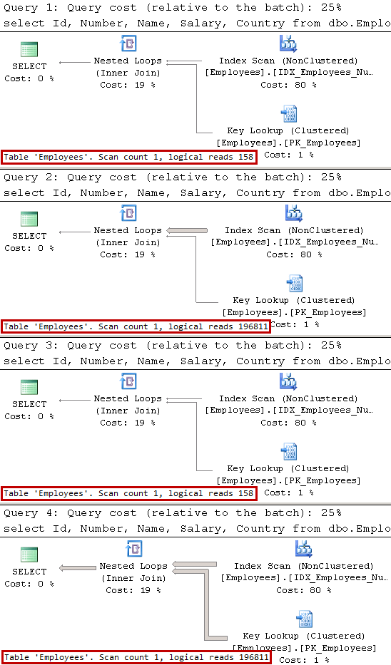
01.Execution Plans When Plans Are Cached

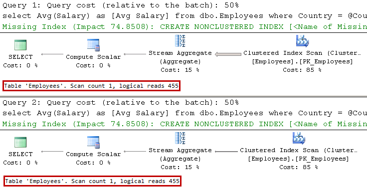
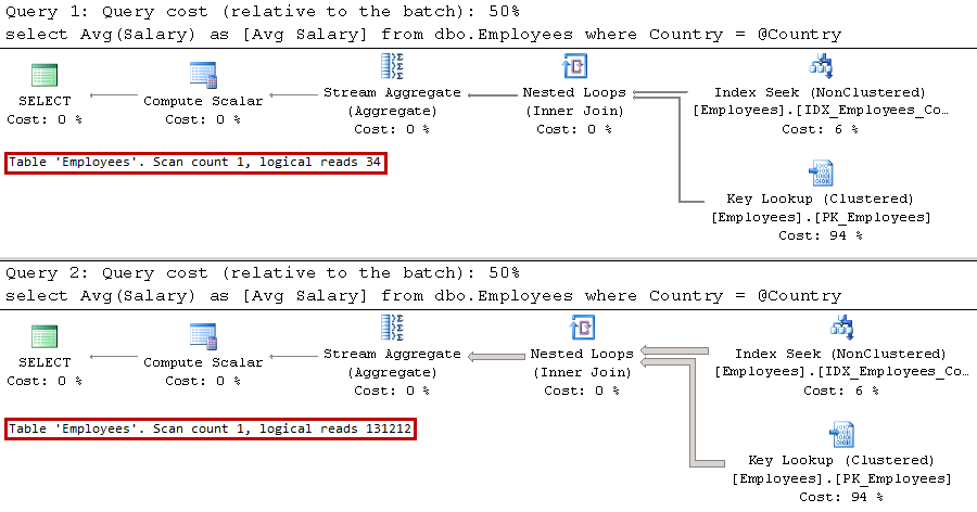
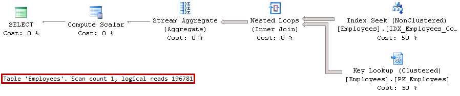
SQL Server compiles stored procedure at time of the first call when only @Number parameter was provided. Even though, the most efficient execution plan for this case is IDX_Employees_Number Index Seek operation, SQL Server cannot cache such execution plan because it would not be valid for the case, when @Number parameter is NULL. Therefore, SQL Server generated and cached execution plan that utilizes Index Scan operation, which is highly inefficient in case, when @Number parameter is not provided. In that case, SQL Server performs Key Lookup operation for every row in the nonclustered index optionally evaluating predicate on @Name parameter afterwards.

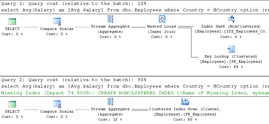
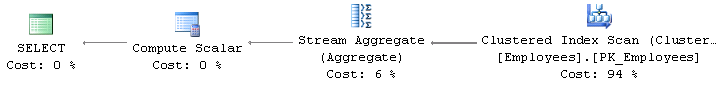
Similar to parameter sniffing issues, you can address this problem with statement-level recompilation as it is shown below. SQL Server recompiles the query on every call, and therefore it can choose the most beneficial execution plan for every parameter set.

It is also worth mentioning that the plans are not cached in cases where statement-level recompile is used.

alter proc dbo.SearchEmployee
(
	@Number varchar(32) = null
	,@Name varchar(100) = null
)
as
begin
	select Id, Number, Name, Salary, Country
	from dbo.Employees
	where 
		((@Number is null) or (Number=@Number)) and
		((@Name is null) or (Name=@Name))
	option (recompile)
end

02.Execution Plans With Statement-Level Recompile

As we already discussed, query recompilation adds CPU overhead. That overhead can be acceptable in case of large and complex queries when compilation time is just the fraction of the query execution time and system is not CPU-bound. In that case, recompilation can even help producing the better execution plans, which would be generated based on the current parameter values, especially if table variables are involved. However, this recompilation overhead is usually not acceptable in case of OLTP queries that are called very often.

One of the options you can use to address the issue is writing multiple queries using IF statements covering all possible combinations of parameters. SQL Server would cache the plan for each statement in the procedure. Listing below shows such an approach, however it quickly becomes unmanageable with a large number of parameters. The number of combinations to cover is equal to the number of parameters squared.

alter proc dbo.SearchEmployee
(
	@Number varchar(32) = null
	,@Name varchar(100) = null
)
as
begin
	if @Number is null and @Name is null
		select Id, Number, Name, Salary, Country
		from dbo.Employees
	else if @Number is not null and @Name is null
		select Id, Number, Name, Salary, Country
		from dbo.Employees
		where Number=@Number
	else if @Number is null and @Name is not null
		select Id, Number, Name, Salary, Country
		from dbo.Employees
		where Name=@Name
	else 
		select Id, Number, Name, Salary, Country
		from dbo.Employees
		where Number=@Number and Name=@Name
end

In the case of a large number of parameters, dynamic SQL becomes the only option. SQL Server will cache the execution plans for each dynamically generated SQL statement. Remember that using dynamic SQL breaks ownership chaining, and it always executes in the security context of CALLER. You should also always use parameters with dynamic SQL to avoid SQL Injection.

alter proc dbo.SearchEmployee
(
	@Number varchar(32) = null
	,@Name varchar(100) = null
)
as
begin
	declare
		@SQL nvarchar(max) = N'	
select Id, Number, Name, Salary, Country
from dbo.Employees
where 1=1'
	
	if @Number is not null
		select @Sql = @SQL + N' and Number=@Number'
	if @Name is not null
		select @Sql = @SQL + N' and Name=@Name'
	exec sp_executesql @Sql, N'@Number varchar(32), @Name varchar(100)'
		,@Number=@Number, @Name=@Name
end

While most of us are aware about danger of using optional parameters and OR predicates in the queries, there is another less known issue associated with filtered indexes. SQL Server will not generate and cache a plan that uses a filtered index, in cases when that index cannot be used with some combination of parameter values.

Listing below shows an example. SQL Server will not generate the plan, which is using the IDX_RawData_UnprocessedData index, even when the @Processed parameter is set to zero because this plan would not be valid for a non-zero @Processed parameter value.

create unique nonclustered index IDX_RawData_UnprocessedData
on dbo.RawData(RecID)
include(Processed)
where Processed = 0;

-- Compiled Plan for the query would not use filtered index
select top 100 RecId, /* Other columns */
from dbo.RawData
where RecID > @RecID and Processed = @Processed
order by RecID;

In that particular case, rewriting the query using IF statement would be, perhaps, the best option.

if @Processed = 0
	select top 1000 RecId, /* Other Columns */
	from dbo.RawData
	where RecId > @RecId and Processed = 0
	order by RecId;
else 
	select top 1000 RecId, /* Other Columns */
	from dbo.Data
	where RecId > @RecId and Processed = 1
	order by RecId;

Unfortunately, IF statement does not always help. In some cases, SQL Server can auto-parametrize the queries and replace some of the constants with auto-generated parameters. That behavior allows SQL Server to reduce the size of the plan cache; however, it could lead to all plan reuse issues we have already discussed.

By default, SQL Server uses SIMPLE parametrization and parametrize only the simple queries. However, if database or query are using FORCED parametrization, that behavior can become the issue. Let’s look at a particular example and create a database with a table with a filtered index and populate it with some data, as shown below.

use master
go

create database ParameterizationTest
go

use ParameterizationTest
go

create table dbo.RawData
(
	RecId int not null identity(1,1), 
	Processed bit not null, 
	Placeholder char(100),
	constraint PK_RawData
	primary key clustered(RecId)
);

/* Inserting:
	Processed = 1: 65,536 rows
	Processed = 0: 16 rows */
;WITH N1(C) AS (SELECT 0 UNION ALL SELECT 0) -- 2 rows
,N2(C) AS (SELECT 0 FROM N1 AS T1 CROSS JOIN N1 AS T2) -- 4 rows
,N3(C) AS (SELECT 0 FROM N2 AS T1 CROSS JOIN N2 AS T2) -- 16 rows
,N4(C) AS (SELECT 0 FROM N3 AS T1 CROSS JOIN N3 AS T2) -- 256 rows
,N5(C) AS (SELECT 0 FROM N4 AS T1 CROSS JOIN N4 AS T2 ) -- 65,536 rows
,IDs(ID) AS (SELECT ROW_NUMBER() OVER (ORDER BY (SELECT NULL)) FROM N5)
insert into dbo.RawData(Processed)
	select 1
	from Ids;

insert into dbo.RawData(Processed)
	select 0
	from dbo.RawData
	where RecId <= 16;

create unique nonclustered index IDX_RawData_Processed_Filtered 
on dbo.RawData(RecId)
include(Processed)
where Processed = 0;

For the next step, let’s run the queries that count a number of unprocessed rows in both SIMPLE and FORCED parametrization modes.

select count(*)
from dbo.RawData
where Processed = 0			
go

alter database ParameterizationTest set parameterization forced
go

select count(*)
from dbo.RawData
where Processed = 0

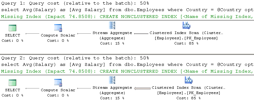
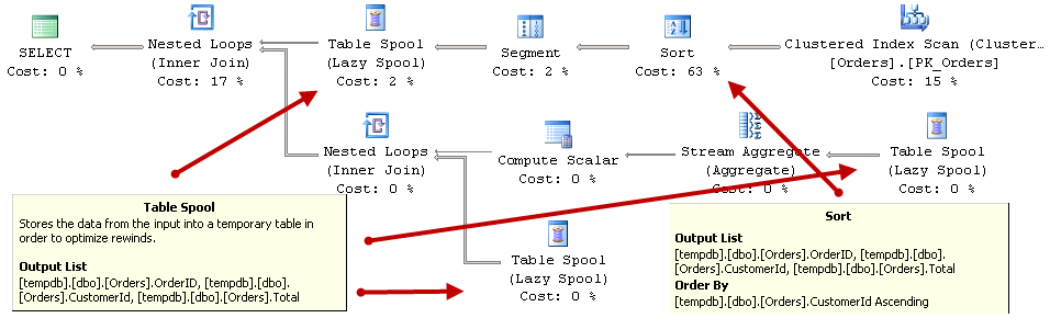
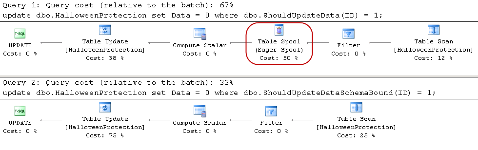
If you examine the execution plans shown in Figure 3, you will notice that SQL Server utilized a filtered index in the case of a SIMPLE parametrization. SQL Server can cache this plan because of the constant in the Processed=0 predicate. Alternatively, with FORCED parametrization, SQL Server parametrizes the query using the parameter in the Processed=@0 predicate. Therefore, it cannot cache the plan with the filtered index because it would not be valid for the case when a query selects processed (Processed=1) rows. SQL Server generated the execution plan with a Clustered Index Scan, which is far less efficient in this case.

03.Execution Plans and Parametrization

The workaround in this case is using SIMPLE parametrization for the database, or forcing it on query level with plan guide (more on it later). In some cases, you would also need to rewrite the query and use one of the constructs that prevent parametrization in SIMPLE parametrization mode, such as IN, TOP, DISTINCT, JOIN, UNION, subqueries and quite a few others.

Plan caching and plan reuse are the great features that help to reduce CPU load on the server. However, they introduce several side effects you need to be aware of and keep them in mind when you write queries and stored procedures.

Source code is available for download

Plan Cache: Parameter Sniffing

There are several reasons why it is beneficial to use parameters in the queries. It mitigates security risks by protecting from SQL Injection. Moreover, it helps with the performance. Query optimization is expensive and resource-intensive process. SQL Server reduces that cost by keeping execution plans in the special part of the memory called Plan Cache and reusing them on subsequent calls.

Even though, this approach benefits the system by reducing the number of query compilations, it could also introduce some issues. Cached plans can become inefficient due to the data distribution and/or parameter values change. SQL Server tracks changes in the data by counting number of changes of the index columns outdating statistics and recompiling queries when number of changes reach about 20% of number of rows in the table (trace flag 2371 can reduce that threshold). However, tracking parameter values change is more complicated.

When SQL Server compiles parametrized query or stored procedure, it analyzes parameters and generates execution plan, which is optimal for those specific values. This process is called Parameter Sniffing. Furthermore, generated plans are cached and reused regardless of parameter values at time of reuse. That behavior can lead to the situations when query is compiled and plan is generated based on atypical parameter set. Cached plan, in this case, would be suboptimal for the calls that reuse that plan.

All of us experienced the situations when query or stored procedure suddenly became very slow even when they ran fine before. Parameter sniffing could be the reason of why it happened. SQL Server decided to recompile the query due to statistics update and the query that triggered recompilation had atypical parameter values. Even though, generated execution plan was efficient for parameters at time of compilation; that cached plan is not necessarily efficient for the other queries that reuses it.

Historically, parameter sniffing has the negative connotation in SQL Server community. It is used to explain why queries have suboptimal execution plans, like I just did in the previous paragraph. This is vastly wrong, however. Parameter sniffing is just the name for SQL Server behavior of analyzing parameters during query compilation.

Let’s look at a few examples of parameter sniffing and discuss how to address the issues it can introduce. In this post, I am using the stored procedure; however, everything would work the same in case of parametrized queries.

As the first step, let’s create a table dbo.Employees. We will populate it distributing data in the way that most rows have Country column value of USA with a few employees with Country value of Canada. Listing below shows the code.

create table dbo.Employees
(
	ID int not null,
	Number varchar(32) not null,
	Name varchar(100) not null,
	Salary money not null,
	Country varchar(64) not null,

	constraint PK_Employees
	primary key clustered(ID)
);

;with N1(C) as (select 0 union all select 0) -- 2 rows
,N2(C) as (select 0 from N1 as T1 cross join N1 as T2) -- 4 rows
,N3(C) as (select 0 from N2 as T1 cross join N2 as T2) -- 16 rows
,N4(C) as (select 0 from N3 as T1 cross join N3 as T2) -- 256 rows
,N5(C) as (select 0 from N4 as T1 cross join N4 as T2 ) -- 65,536 rows
,Nums(Num) as (select row_number() over (order by (select null)) from N5)
insert into dbo.Employees(ID, Number, Name, Salary, Country)
	select 
		Num, 
		convert(varchar(5),Num), 
		'USA Employee: ' + convert(varchar(5),Num), 
		40000,
		'USA'
	from Nums;

;with N1(C) as (select 0 union all select 0) -- 2 rows
,N2(C) as (select 0 from N1 as T1 cross join N1 as T2) -- 4 rows
,N3(C) as (select 0 from N2 as T1 cross join N2 as T2) -- 16 rows
,Nums(Num) as (select row_number() over (order by (select null)) from N3)
insert into dbo.Employees(ID, Number, Name, Salary, Country)
	select 
		65536 + Num, 
		convert(varchar(5),65536 + Num), 
		'Canada Employee: ' + convert(varchar(5),Num), 
		40000,
		'Canada'
	from Nums;

create nonclustered index IDX_Employees_Country
on dbo.Employees(Country);

As a next step, let’s create a stored procedure that calculates the average salary for employees in a specific country.

create proc dbo.GetAverageSalary @Country varchar(64)
as
begin
	select Avg(Salary) as [Avg Salary]
	from dbo.Employees
	where Country = @Country
end

As you can guess, when we call this stored procedure with parameter @Country=’USA’, stored procedure needs to touch almost every row in the table and the most optimal execution plan is Clustered Index Scan. However, when we call the stored procedure with parameter @Country=’Canada’, the most efficient execution plan is Nonclustered Index Seek with Key Lookup operators.

Let’s call the stored procedure twice: the first time with @Country=’USA’ and the second time with @Country=’Canada’, as shown below.

exec dbo.GetAverageSalary @Country='USA';
exec dbo.GetAverageSalary @Country='Canada';

As you can see in Figure 1, SQL Server compiles the stored procedure and caches the plan with the first call and reuses it later. Even though such a plan is less efficient with the @Country=’Canada’ parameter value, it may be acceptable when those calls are rare, which is expected with such a data distribution.

01. Execution plans when the stored procedure is compiled with @Country=’USA’

Now let’s take a look what happens if we swap those calls when the plan is not cached. We will use the DBCC FREEPROCCACHE command, which clears plan cache (DO NOT RUN IT ON PRODUCTION SERVER). As I already mentioned, another instance when this might happen is with a statistics update that forces query to recompile.

dbcc freeproccache
go

exec dbo.GetAverageSalary @Country='Canada';
exec dbo.GetAverageSalary @Country='USA';

As you can see in Figure 2, SQL Server now caches the plan based on the @Country=’Canada’ parameter value. Even though this plan is more efficient when the stored procedure is called with @Country=’Canada’, it is highly inefficient for @Country=’USA’ calls.

02. Execution plans when the stored procedure is compiled with @Country=’Canada’

There are a few ways to address the issue. You can force the recompilation of either stored procedure using EXECUTE WITH RECOMPILE or a statement-level recompile with OPTION (RECOMPILE) clauses. Obviously, a statement-level recompile is better because it performs the recompilation on a smaller scope. SQL Server sniffs the parameter values at the time of the recompilation, generating the optimal execution plan for each parameter value. It is also worth mentioning, that statement-level recompile allows SQL Server to obtain number of rows stored in table variables, which can help to generate more efficient execution plans in some cases.

alter proc dbo.GetAverageSalary @Country varchar(64)
as
begin
	select Avg(Salary) as [Avg Salary]
	from dbo.Employees
	where Country = @Country
	option (recompile)
end
go

exec dbo.GetAverageSalary @Country='Canada';
exec dbo.GetAverageSalary @Country='USA';

As you can see in Figure 3, SQL Server recompiles the statement on every call, and it generates the most efficient execution plan for every parameter value. It is also worth noting that SQL Server does not cache plans for the statements when statement-level recompile is used.

03. Execution plans with OPTION (RECOMPILE) hint

The statement-level recompile may be a good option when the queries do not execute very often or in the case of complex queries, when the compilation time is just a fraction of the total execution time. However, it is hardly the best approach for OLTP queries, which are constantly running in the system due to the extra CPU load that recompilation introduces.

Another option is using an OPTIMIZE FOR hint, which forces SQL Server to optimize a query for the specific parameter values provided in the hint. Listing below illustrates such an approach.

alter proc dbo.GetAverageSalary @Country varchar(64)
as
begin
	select Avg(Salary) as [Avg Salary]
	from dbo.Employees
	where Country = @Country
	option (optimize for(@Country='USA'))
end
go

exec dbo.GetAverageSalary @Country='Canada';
exec dbo.GetAverageSalary @Country='USA';

As you can see in Figure 4, SQL Server ignores the parameter value during the compilation and optimizes the query for the @Country=’USA’ value.

04. Execution plans with OPTIMIZE FOR hint

Unfortunately, the OPTIMIZE FOR hint introduces supportability issues, and it can lead to suboptimal execution plans in cases where the data distribution has changed. Let’s consider the situation, albeit unrealistic, when a company and all of its employees moved from the United States to Germany.

update dbo.Employees set Country='Germany' where Country='USA';

exec dbo.GetAverageSalary @Country='Germany';

Statistics are outdated at the time of the update, which forces SQL Server to recompile the statement in the stored procedure. At this point, there are no rows in the table with Country=’USA’, and the recompilation produces a suboptimal execution plan, as shown in Figure 5. As a side note, the query uses more reads than before due to the index fragmentation introduced by the update.

05. Inefficient execution plan after data distribution change

SQL Server 2008 introduced another optimization hint, OPTIMIZE FOR UNKNOWN, which helps to address such situations. With this hint, SQL Server performs an optimization based on the most statistically common value in the table. Listing below shows the code involved in doing this.

alter proc dbo.GetAverageSalary @Country varchar(64)
as
begin
	select Avg(Salary) as [Avg Salary]
	from dbo.Employees
	where Country = @Country
	option (optimize for(@Country UNKNOWN))
end
go

exec dbo.GetAverageSalary @Country='Canada';

Figure 6 illustrates the execution plan. Country=’Germany’ is the most statistically common value in the table, and therefore SQL Server generates an execution plan that is optimal for such a parameter value.

06. Execution plan with OPTIMIZE FOR UNKNOWN hint

You can achieve the same results with an OPTIMIZE FOR UNKNOWN hint by using local variables instead of parameters. This method also works with SQL Server 2005, where the OPTIMIZE FOR UNKNOWN hint is not supported. Listing below illustrates that approach. It introduces the same execution plan with a Clustered Index Scan, as shown in Figure 6 above.

alter proc dbo.GetAverageSalary @Country varchar(64)
as
begin
	declare
		@CountryTmp varchar(64)
	set @CountryTmp = @Country

	select Avg(Salary) as [Avg Salary]
	from dbo.Employees
	where Country = @CountryTmp
end

Finally, in case when you are dealing with 3rd party systems and cannot add optimization hints to the code, you could use plan guides to achieve the same goal. We will discuss plan guides in one of the future blog posts.

Source code is available for download.

Partial Database Backup and Piecemeal Restore in Microsoft SQL Server

Unfortunately, disasters happen. Regardless of how good is High Availability strategy that you have implemented, there is always the chance that one day you will need to move the database to another server and quickly bring system online. And the chance is – you will have to do it under stress with your phone ringing every few minutes and your manager asking about ETA. It does not help that such process can be very time consuming in the case of the large databases.

Enterprise Edition of SQL Server supports concept of piecemeal restore and allows you to restore database on filegroup-by-filegroup basis keeping database online during the process. Queries that access data from online filegroups would work just fine. This is the great technique that can dramatically reduce system downtime.

In the large number of cases, the size of the operational data that is required for system to be operational is relatively small. Historical data, on the other hand, is often kept due to regulation/compliance reasons and rarely accessed by the applications. As you can guess, it allows you to quickly bring part of the database that supports operational activity online and work with remaining historical data afterwards while customers can connect and use the system.

Obviously, you should design data placement in the way that supports piecemeal restore. In the nutshell, it means the separation of the operational and historical data across different filegroups. As the example, let’s consider Order Entry/Shopping Cart system that stores data for several years. One of the data layout designs could be the following:

  • Empty Primary FG. Primary Filegroup should be online in order for database to be online. It is good idea to keep primary filegroup empty and do not place any objects there.
  • Entities FG. This filegroup could store catalog tables, such as Customers, Articles and others.
  • One or more filegroups for the operational data. For example, if operational period is the current year, this filegroup can store Orders, OrderLineItems and related entities that stores current-year data.
  • One or more filegroups for the historical data. Those filegroups store data that is not required to support operational activity in the system.

Piecemeal restore strategy will require you to bring online Primary, Entities and Operation data filegroups first. System will be available to the customers at this point. After that, you can work on restoring historical data filegroups, which in most part of the cases, will be significantly larger than operational data and, therefore, will take longer time to restore.

It is also worth noting, that in case of SQL Server 2014 In-memory OLTP, you should also have Hekaton filegroup online before database becomes available to the users. Usually, In-memory tables keep operational data anyway, so it should not be a problem in most part of the cases.

Let’s look at the example and create a database with the structure outlined above. For simplicity sake, every filegroup has only one data file. However, in the real-life you should consider creating multiple files to reduce allocation contention in the filegroups with volatile data.

create database [MyBigOrderDb]
on primary
(name = N'MyBigOrderDb', filename = N'c:\db\MyBigOrderDb.mdf'), 
filegroup [Entities] 
(name = N'MyBigOrderDB_Entities', filename = N'c:\db\MyBigOrderDB_Entities.ndf'), 
filegroup [FG2013] 
(name = N'MyBigOrderDB_FG2013', filename = N'c:\db\MyBigOrderDB_FG2013.ndf'), 
filegroup [FG2014] 
(name = N'MyBigOrderDB_FG2014', filename = N'c:\db\MyBigOrderDB_FG2014.ndf')
log on
(name = N'MyBigOrderDb_log', filename = N'c:\db\MyBigOrderDb_log.ldf')

As the next step, let’s create a few tables including partitioned table Orders.

create table dbo.Customers
(
    CustomerId int not null,
    CustomerName nvarchar(64) not null,
)
on [Entities];

create table dbo.Articless
(
 ArticlesId int not null,
 ArticleName nvarchar(64) not null,
)
on [Entities];

create partition function pfOrders(smalldatetime)
as range right
for values('2014-01-01');

create partition scheme psOrders
as partition pfOrders
to (FG2013,FG2014)
go

create table dbo.Orders
(
    OrderId int not null,
    OrderDate smalldatetime not null,
    OrderNum varchar(32) not null,
    constraint PK_Orders
    primary key clustered(OrderDate, OrderId)
    on psOrders(OrderDate)
)
go

insert into dbo.Customers(CustomerId, CustomerName) values(1,'Customer 1');
insert into dbo.Orders(OrderDate, OrderId, OrderNum)
values
    ('2013-01-01',1,'Order 1'),
    ('2013-02-02',2,'Order 2'),
    ('2014-01-01',3,'Order 3'),
    ('2014-02-02',4,'Order 4')

Next, let’s create the backup chain and perform FULL, DIFFIRENTIAL and LOG backups.

-- Full backup
backup database [MyBigOrderDb] 
to disk = N'c:\db\MyBigOrderDb_Full.bak' 
with noformat, init, name = N'MyBigOrderDb-Full Database Backup', 
    compression, stats = 2
go

-- Differential backup
backup database [MyBigOrderDb] 
to disk = N'c:\db\MyBigOrderDb_Diff.bak' 
with differential, noformat, init, 
    name = N'MyBigOrderDb-Differential Database Backup', 
    compression, stats = 2
go

-- Transaction log
backup log [MyBigOrderDb] 
to disk = N'c:\db\MyBigOrderDb_Log.trn' 
with noformat, init, name = N'MyBigOrderDb-Tran Log', 
    compression, stats = 2
go

And at this point, let’s assume that disaster happens and we need to move database to another server. In this example, I would assume that we still have access to transaction log of the original database and we will perform tail-log backup to avoid any data loss.

backup log [MyBigOrderDb] 
to disk = N'c:\db\MyBigOrderDb_TailLog.trn' 
with no_truncate, noformat, init, name = N'MyBigOrderDb-Tail Log', 
 compression, norecovery, stats = 2

At this point, we will need to copy all files from the backup chain to another server and start restore process. We will perform piecemeal restore of Primary, Entities and FG2014 filegroups to support operational activity of the system without bringing historical FG2013 data online. The first operation is performing restore of the FULL database backup specifying just the filegroups we need to restore.

-- Restoring on another server (Same folder structure for demo sake)
-- Full Backup
restore database [MyBigOrderDb] 
FILEGROUP = 'primary', FILEGROUP = 'Entities', FILEGROUP = 'FG2014'
from disk = N'C:\DB\MyBigOrderDb_Full.bak' with file = 1,
move N'MyBigOrderDB' to N'c:\db\MyBigOrderDb.mdf', 
move N'MyBigOrderDB_Entities' to N'c:\db\MyBigOrderDb_Entities.ndf', 
move N'MyBigOrderDB_FG2014' to N'c:\db\MyBigOrderDb_2014.ndf', 
move N'MyBigOrderDb_log' to N'c:\db\MyBigOrderDb.ldf', 
NORECOVERY, partial, stats = 2;

it is worth mentioning, that I am using WITH NORECOVERY clause in all RESTORE commands including tail-log backup restore. In the end, I am recovering database with the separate RESTORE statement. This is just a good practice and safety measurement. By default, Management Studio uses WITH RECOVERY option with restore, which can lead to the situation that you accidentally recovered database at intermediate restore stage. You would not be able to restore further backups after that and would be forced to start from scratch.

As the next steps, we need to restore DIFFERENTIAL, LOG and tail-log backups as shown below. You do not need to specify filegroups as part of restore statement anymore – SQL Server would perform restore only in scope of the filegroups we are working with and which are in RESTORING state.

-- Diff Backup
restore database [MyBigOrderDb] 
from disk = N'C:\DB\MyBigOrderDb_Diff.bak' with file = 1,
NORECOVERY, stats = 2;

-- Tran Log
restore database [MyBigOrderDb] 
from disk = N'C:\DB\MyBigOrderDb_Log.trn' with file = 1,
NORECOVERY, stats = 2;

-- Tail-log
restore database [MyBigOrderDb] 
from disk = N'C:\DB\MyBigOrderDb_TailLog.trn' with file = 1,
NORECOVERY, stats = 2;

-- Recovery
restore database [MyBigOrderDb] with RECOVERY;

At this point, our database is partially online. We can query operational data as it shown below in Figure 1.

select * from MyBigOrderDb.dbo.Customers
select * from MyBigOrderDb.dbo.Orders where OrderDate >= '2014-01-01'

01. Querying Data from Operational Filegroups

However, if we try to query historical data, we will get an error, as shown in Figure 2

select * from MyBigOrderDb.dbo.Orders where OrderDate < '2014-01-01'

02. Querying Data from Historical Filegroup

You can check the status of the database filegroups with the following query. Figure 3 shows that three filegroups are online while FG2013 filegroup is still in RECOVERY_PENDING stage.

select file_id, name, state_desc, physical_name
from MyBigOrderDb.sys.database_files

03. Filegroup Status Before Historical Filegroup Restore

As you see, customers can use the system while we are working on restoring of FG2013 filegroup. We can perform this with the following script:

-- Full Backup (restoring individual filegroup)
restore database [MyBigOrderDb] 
FILEGROUP = 'FG2013'
from disk = N'C:\DB\MyBigOrderDb_Full.bak' with file = 1,
move N'MyBigOrderDB_FG2013' to N'c:\db\MyBigOrderDb_2013.ndf',  
stats = 2;

-- Diff Backup
restore database [MyBigOrderDb] 
from disk = N'C:\DB\MyBigOrderDb_Diff.bak' with file = 1,
stats = 2;

-- Tran Log
restore database [MyBigOrderDb] 
from disk = N'C:\DB\MyBigOrderDb_Log.trn' with file = 1,
stats = 2;

-- Tail-log
restore database [MyBigOrderDb] 
from disk = N'C:\DB\MyBigOrderDb_TailLog.trn' with file = 1,
stats = 2;

Now database is online as it is shown in Figure 4.

04. Filegroups Status After Historical Filegroup Restore

Piecemeal restore can significantly decrease database restore time. However, there is still time-consuming part in this process. Regardless how many filegroups you are restoring, you should copy/move backup file that contains initial FULL database backup to the new server. Time of this operation depends on network throughput and slow network and/or large backup files can lead to very long delays.

Obviously, you can take several approaches. You can always “be prepared” and copy files to reserved server after each backup. With such strategy, you would already have backup files in place when they need to be restored if/when disaster occurs.

However, you can use another approach if historical data is read-only. This approach is called “partial database backup”. Even though, Microsoft stated that it is designed for SIMPLE recovery models, it would work just fine with FULL recovery model, as long as you implemented it correctly.

Let’s look how it works and as the first step, let’s mark our FG2013 filegroup as read-only:

alter database MyBigOrderDb modify filegroup FG2013 readonly

At this point, you should start the new backup chain, which, in the nutshell, are two different sets of backup files. One set includes backup files for read-write filegroups (FULL, DIFFERENTIAL and LOG backups using READ_WRITE_FILEGROUPS option. In addition, you need to perform backup of read-only filegroup. You can do it with the script shown below:

-- Backing Up Read-Only Filegroup
backup database [MyBigOrderDb] 
FILEGROUP = N'FG2013'
to disk = N'c:\db\MyBigOrderFG2013.bak' 
with noformat, init, 
	name = N'MyBigOrderDb-FG2013 FG backup', 
	compression, stats = 2
go

-- Full backup of read_write filegroups
backup database [MyBigOrderDb] READ_WRITE_FILEGROUPS
to disk = N'c:\db\MyBigOrderDbRW_Full.bak' 
with noformat, init, name = N'MyBigOrderDb-Full Database Backup (R/W FG)', 
	compression, stats = 2
go

-- Differential backup
backup database [MyBigOrderDb] 
to disk = N'c:\db\MyBigOrderDbRW_Diff.bak' 
with differential, noformat, init, 
	name = N'MyBigOrderDb-Differential Database Backup (R/W FG)', 
	compression, stats = 2
go

-- Transaction log
backup log [MyBigOrderDb] 
to disk = N'c:\db\MyBigOrderDbRW_Log.trn' 
with noformat, init, name = N'MyBigOrderDb-Tran Log', 
	compression, stats = 2

The beauty of this situation that now you have data backups separated. You would have relatively small backup chain file(s) for operational data as well as large static backup file for read-only historical data. This will dramatically reduce time required to move operational data backup files over network.  It also helps with day-to-day backup strategy and reduces the time of backup operation and, server and network load, and storage space required to store the files. You can create new backup chains of operation data without taking new backup for historical data as long as those filegroups stay read-only.

If disaster occurs and you need to move database to another server, you can start with operation data backup chain as shown below. For simplicity sake, I am omitting tail-log backup – however, in real life you should always obtain it to avoid data loss.

-- Restoring on another server (Same folder structure for demo sake)
-- Full Backup (R/W filegroups only)
restore database [MyBigOrderDb] 
filegroup = 'primary', filegroup = 'Entities', filegroup = 'FG2014'
from disk = N'C:\DB\MyBigOrderDbRW_Full.bak' with file = 1,
move N'MyBigOrderDB' to N'c:\db\MyBigOrderDb.mdf',  
move N'MyBigOrderDB_Entities' to N'c:\db\MyBigOrderDb_Entities.ndf',  
move N'MyBigOrderDB_FG2014' to N'c:\db\MyBigOrderDb_2014.ndf',  
move N'MyBigOrderDb_log' to N'c:\db\MyBigOrderDb.ldf',  
norecovery, partial, stats = 2;

-- Diff Backup
restore database [MyBigOrderDb] 
from disk = N'C:\DB\MyBigOrderDbRW_Diff.bak' with file = 1,
norecovery, stats = 2;

-- Tran Log
restore database [MyBigOrderDb] 
from disk = N'C:\DB\MyBigOrderDbRW_Log.trn' with file = 1,
norecovery, stats = 2;

-- Recovery
restore database [MyBigOrderDb] with recovery;

If you queried the status of the database filegroups after restore, you would see very similar picture – all operational filegroups are online and historical filegroup is in RECOVERY_PENDING state. Figure 5 illustrates that.

05. Filegroup Status During Partial Restore

Again, at this point system is available to users and you can continue working on historical data while system is operational with the following script.

-- Restoring Read/Only Filegroup
restore database [MyBigOrderDb] 
filegroup = 'FG2013'
from disk = N'C:\DB\MyBigOrderFG2013.bak' with file = 1,
move N'MyBigOrderDB_FG2013' to N'c:\db\MyBigOrderDb_2013.ndf',  
recovery, stats = 2;

Be careful when you change read-only status of the filegroups when partial backup is used. One of examples of such scenario is when operational period changed and you need to move some former-operational data that becomes historical to another filegroup. One of the approaches to accomplish it is making historical filegroup as read-write, copying data there and making it read-only again. You can still restore the database using old read-only filegroup backup as long as you have backup chain with LOG backups that cover data movement operations. However, you would not be able to recover historical data if you start new backup chain for updateable filegroups after the fact and did not take new backup of the read-only filegroup.

As the general recommendation, it is safer to start new backup chain together with backup of historical filegroup after you made historical filegroup read-only again. And, most importantly, regardless what solution you are using, test your backup and restore strategies. This would help you to avoid unpleasant surprises when things went south.

Writing Triggers in the Right Way

The only correct way of writing triggers is not writing them. I would repeat – the only correct way of writing triggers is not writing them. Triggers negatively affect performance. AFTER triggers introduce fragmentation and increase tempdb load due to version store usage. Triggers are running in context of transaction, increase the time in which locks are held and contribute to locking and blocking in the system. However, in some cases, we have to use triggers and it is important to develop them correctly.

SQL Server fires triggers on statement rather than row level. For example, if update statement modified 10 rows, AFTER UPDATE and/or INSTEAD OF UPDATE trigger would fire once rather than 10 times. Therefore, trigger must handle situations when inserted and/or deleted tables have multiple rows.  Let’s look at the example and create a table with AFTER INSERT trigger as shown below:

create table dbo.Data 
( 
	ID int not null, 
	Value varchar(32) 
) 
go 

create trigger trgData_AI on dbo.Data 
after insert 
as 
	/* Some code */ 
	declare 
		@ID int 
	set @ID = (select ID from inserted) 
	/* Some code */

Everything is fine when you inserted a single row. However, multi-row insert would fail with exception shown below.

Msg 512, Level 16, State 1, Procedure trgData_AI, Line 9
Subquery returned more than 1 value. This is not permitted when the subquery follows =, !=, <, <= , >, >= or when the subquery is used as an expression.
The statement has been terminated.

And there is another consequence of statement-level nature of triggers. They fire even if DML statement did not modify any rows. Would it introduce any issues in the system or not depends on implementation. However, it would always lead to unnecessary performance overhead.

Let’s look at example. The code below creates another table and changes trigger in a way, that mimics behavior of audit functional, which is frequently implemented based on triggers.

create table dbo.Audit 
( 
	ID int not null identity(1,1), 
	OnDate datetime2(0) not null 
		constraint DEF_Audit_OnDate  
		default getutcdate(), 
	Message varchar(64) not null, 
)
go

alter trigger trgData_AI on dbo.Data 
after insert 
as 
begin
	declare 
		@Msg varchar(64) = 'Triggers are bad. And @@ROWCOUNT=' + convert(varchar(10),@@rowcount) 

	insert into dbo.Audit(Message) values(@Msg); 
end

Now let’s run insert statement, which does not insert any rows to the table.

insert into dbo.Data(ID, Value) 
	select 1, 'ABC'  
	where 1 = 0

If you checked content of Audit table, you would see that trigger was fired:

01. Content of Audit table

So the first important conclusion is that every trigger must checks @@ROWCOUNT variable as the very first statement in implementation.

SET NOCOUNT ON should be the second action trigger does. Without that SQL Server returns affected number of rows for each operator in the trigger in addition to original DML statement. Some client libraries rely on the single message in the output and would not work correctly in case of multiple messages. Therefore, the first two statements in the trigger should look like it is shown below.

alter trigger trgData_AI on dbo.Data 
after insert 
as 
begin
	if @@ROWCOUNT = 0
		return
	set nocount on

	/* Some Code Here */
end

Finally, there is another caveat. While implementation above works for insert, update and delete operators, it is not the case with merge@@ROWCOUNT in this case represents total number of rows affected by merge statement rather than by individual insert, update or delete action in the trigger. Let’s prove it with the example.

create table dbo.Data2(Col int not null)
go

create trigger trg_Data_AI on dbo.Data2
after insert 
as
	select 
		'After Insert' as [Trigger]
		,@@RowCount as [RowCount]
		,(select count(*) from inserted) as [Inserted Cnt]
		,(select count(*) from deleted) as [Deleted Cnt]
go

create trigger trg_Data_AU on dbo.Data2
after update
as
	select 
		'After Update' as [Trigger]
		,@@RowCount as [RowCount]
		,(select count(*) from inserted) as [Inserted Cnt]
		,(select count(*) from deleted) as [Deleted Cnt]
go

create trigger trg_Data_AD on dbo.Data2
after delete
as
	select 
		'After Delete' as [Trigger]
		,@@RowCount as [RowCount]
		,(select count(*) from inserted) as [Inserted Cnt]
		,(select count(*) from deleted) as [Deleted Cnt]
go

Now let’s run MERGE statement as shown below:

merge into dbo.Data2 as Target
using (select 1 as [Value]) as Source
on Target.Col = Source.Value
when not matched by target then
	insert(Col) values(Source.Value)
when not matched by source then
	delete
when matched then
	update set Col = Source.Value;

The table is empty, therefore only one insert statement would be executed. However, as you should see below, all three triggers were fired, It is worth mentioning that previous code example demonstrated very bad practice of returning result sets from trigger. You should avoid doing it in production code.

02. Triggers and MERGE statement

The right way to deal with such situation is checking content of inserted and deleted tables as shown below.

alter trigger trg_Data_AI on dbo.Data2
after insert 
as
	if @@rowcount = 0 
		return
	set nocount on
	if exists(select * from inserted)
		/* Some Code Here */      
go

alter trigger trg_Data_AU on dbo.Data2
after update
as
	if @@rowcount = 0 
		return
	set nocount on
	if	exists(select * from inserted) and 
		exists(select * from deleted)
		/* Some Code Here */      
go

alter trigger trg_Data_AD on dbo.Data2
after delete
as
	if @@rowcount = 0 
		return
	set nocount on
	if	exists(select * from deleted)
		/* Some Code Here */

I hope that those tips will help you to write trigger in the most optimal way. However, I would repeat – the best way of writing triggers is not writing them at all.

Unwinding Table Spools

One of the questions I have often been asked during various SQL Server events is what exactly Table Spool operator does in execution plan. I would try to answer it today.

Spool operators, in the nutshell, are internal in-memory or on-disk caches/temporary tables. SQL Server often uses spools for performance reasons to cache results of complex subexpressions that needs to be used multiple times during query execution.

Let’s look at the example and create the table, which stores some sales information as shown below:

create table dbo.Orders
(
    OrderID int not null,
    CustomerId int not null,
    Total money not null,
    constraint PK_Orders
    primary key clustered(OrderID)
);

;with N1(C) as (select 0 union all select 0) -- 2 rows
,N2(C) as (select 0 from N1 as T1 cross join N1 as T2) -- 4 rows
,N3(C) as (select 0 from N2 as T1 cross join N2 as T2) -- 16 rows
,N4(C) as (select 0 from N3 as T1 cross join N3 as T2) -- 256 rows
,Nums(Num) as (select row_number() over (order by (select null)) from N4)
    insert into dbo.Orders(OrderId, CustomerId, Total)
        select Num, Num % 10 + 1, Num
        from Nums;

Now let’s run the query that returns the list of orders with the information about total amount of sales on per-customer basis.

select OrderId, CustomerID, Total
	,Sum(Total) over(partition by CustomerID) as [Total Customer Sales] 
from dbo.Orders

As you see, in the execution plan below, SQL Server scans the table, sorts the data based on CustomerID order and uses Table Spool operator to cache the results. It allows SQL Server to access the cached data and avoid expensive sorting operation later.

01. Execution Plan with Spool operators

Even though Table Spool operator is shown in the execution plan multiple times, it is essential the same spool/cache. SQL Server builds it the first time and using its data later.

Technically speaking, there are two different logical spool operators – Eager Spool and Lazy Spool. The only difference between them are how data is populated. With Eager Spool, SQL Server fetches all rows as soon as spool is called. With Lazy Spool, SQL Server fetches rows on demand – when they are needed.

SQL Server also uses spools for Halloween Protection when modifying the data. Halloween Protection helps to avoid situations when data modifications affect what data need to be updated. The classic example of such situation is shown below. Without Halloween Protection, insert statement would fall into infinitive loop, reading rows it has been inserting.

create table dbo.HalloweenProtection
(
	Id int not null identity(1,1),
	Data int not null
);

insert into dbo.HalloweenProtection(Data)
	select Data from dbo.HalloweenProtection;

As you can see in the execution plan of insert statement, SQL Server uses Table Spool operator to cache the data from table as of before insert starts to avoid infinitive loop during execution.

02. Halloween Protection and Table Spools.

Halloween Protection has very interesting side-effect when we are talking about multi-statement user-defined functions (both, scalars and table-valued). Using multi-statement functions is bad practice by itself, however creating them without SCHEMABINDING option is even worse. That option forces SQL Server to analyze if user-defined function performs data access and avoid extra Halloween Protection-related Spool operators in the execution plan.

Let’s see the example and create two user-defined functions and using them in where clause of update statements.

create function dbo.ShouldUpdateData(@Id int)
returns bit
as
begin
	return (1)
end
go

create function dbo.ShouldUpdateDataSchemaBound(@Id int)
returns bit
with schemabinding
as
begin
	return (1)
end
go

update dbo.HalloweenProtection
set Data = 0
where dbo.ShouldUpdateData(ID) = 1;

update dbo.HalloweenProtection
set Data = 0
where dbo.ShouldUpdateDataSchemaBound(ID) = 1;

Neither of functions access the data and therefore can introduce Halloween effect. However, SQL Server does not know that in case of non-schema bound function and add Spool operator to execution plan as shown below.

03. Execution Plans for user-defined functions

Bottom line – you should always make functions schema-bound when you create them.

Spool temporary tables are usually referenced as worktables in I/O statistics for the queries. You should analyze table spool-related reads during query performance tuning. While spools can improve performance of the queries, there is the overhead introduced by unnecessary spools. You can often remove them by creating appropriate indexes on the tables.

SQL Server Storage Engine: Heap Tables

Heap tables are tables without a clustered index. The data in heap tables is unsorted.  SQL Server does not guarantee nor maintain any sorting order of the data in the heap tables.
When we insert data into heap tables, SQL Server tries to fill pages as much as possible, although it does not analyze the actual free space available on a page. It uses the Page Free Space (PFS) allocation map instead. SQL Server errs on the side of caution, and it uses the low value from the PFS free space percentage tier during the estimation.

For example, if a data page stores 4,100 bytes of data, and, as result, has 3,960 bytes of free space available, PFS would indicate that the page is 51-80 percent full. SQL Server would not put a new row to the page if its size exceeds 20 percent (8,060 bytes * 0.2 = 1,612 bytes) of the page size.

Let’s look at the example and create the table with the code shown below.

create table dbo.Heap(Val varchar(8000) not null);

;with CTE(ID,Val) as 
(
    select 1, replicate('0',4089)
    union all
    select ID + 1, Val from CTE where ID < 20 
) 
insert into dbo.Heap(Val)
   select Val from CTE;

select page_count, avg_record_size_in_bytes, avg_page_space_used_in_percent
from sys.dm_db_index_physical_stats(db_id(),object_id(N'dbo.Heap'),0,null,'DETAILED');

01. Page Count after initial insert

At this point, the table stores 20 rows of 4,100 bytes each. SQL Server allocates 20 data pages—one page per row—with 3,960 bytes available. PFS would indicate that pages are 51-80 percent full.

As the next step, let’s inserts the small 111-byte row, which is about 1.4 percent of the page size. As a result, SQL Server knows that the row would fit into one of the existing pages (they all have at least 20 percent of free space available), and a new page should not be allocated.

insert into dbo.Heap(Val) values(replicate('1',100));

select page_count, avg_record_size_in_bytes, avg_page_space_used_in_percent 
from sys.dm_db_index_physical_stats(db_id(),object_id(N'dbo.Heap'),0,null,'DETAILED');

02. Page Count after insertion of small row

Lastly, the third insert statement needs 2,011 bytes for the row, which is about 25 percent of the page size. SQL Server does not know if any of the existing pages have enough free space to accommodate the row and, as a result, allocates the new page. You can see that SQL Server does not access existing pages by checking the actual free space and uses PFS data for the estimation.

insert into dbo.Heap(Val) values(replicate('2',2000));

select page_count, avg_record_size_in_bytes, avg_page_space_used_in_percent 
from sys.dm_db_index_physical_stats(db_id(),object_id(N'dbo.Heap'),0,null,'DETAILED');

03. Page Count after insertion of large row

That behavior leads to the situation where SQL Server unnecessarily allocates new data pages, leaving large amount of free space unused. It is not always a problem when the size of rows vary—in those cases, SQL Server eventually fills empty spaces with the smaller rows. However, especially in cases when all rows are relatively large, you can end up with large amounts of wasted space.

When selecting data from the heap table, SQL Server uses as Index Allocation Map (IAM) to find the pages and extents that need to be scanned. It analyzes what extents belong to the table and processes them based on their allocation order rather than on the order in which the data was inserted. You can see it in figure below.

04. IAM Scan

When you update the row in the heap table, SQL Server tries to accommodate it on the same page. If there is no free space available, SQL Server moves the new version of the row to another page and replaces the old row with a special 16-byte row called a forwarding pointer. The new version of the row is called forwarded row.

05. Forwarding Pointers

There are two main reasons why forwarding pointers are used. First, they prevent updates of nonclustered index keys, which referencing the row.

In addition, forwarding pointers helps minimize the number of duplicated reads – the situation when a single row is read multiple times during the table scan. As the example, let’s look at figure above and assume that SQL Server scans the pages in left-to-right order. Next, let’s assume that the row in page 3 was modified after the page was read at the time when SQL Server reads page 4. The new version of the row would be moved to page 5, which has yet to be processed. Without forwarding pointers, SQL Server would not know that the old version of the row had already been read, and it would read it again during the page 5 scan. With forwarding pointers, SQL Server would ignore the forwarded rows.

Forwarding pointers help minimize duplicated reads at cost of additional read operations. SQL Server follows the forwarding pointers and reads the new versions of the rows at the time it encounters them. That behavior can introduce an excessive number of I/O operations.

Let’s create the table and insert three rows there.

create table dbo.ForwardingPointers
(
   ID int not null,
   Val varchar(8000) null
);

insert into dbo.ForwardingPointers(ID,Val)
values
   (1,null),
   (2,replicate('2',7800)),
   (3,null);

select page_count, avg_record_size_in_bytes, avg_page_space_used_in_percent, forwarded_record_count
from sys.dm_db_index_physical_stats(db_id(),object_id(N'dbo.ForwardingPointers'),0,null,'DETAILED');

set statistics io on
select count(*) as [RowCnt] from dbo.ForwardingPointers
set statistics io off

You can see results below

06. Forwarding Pointers: I/O without forwarding pointers

All three rows fit into the single page, and SQL Server needs to read just that page when it scans the table.

07. Page Layout without Forwarding Pointers

Let’s update two of the table rows and increase their size. The new version of the rows would not fit into the page anymore, which introduces the allocation of the two new pages and two forwarding pointers.

update dbo.ForwardingPointers set Val = replicate('1',5000) where ID = 1;
update dbo.ForwardingPointers set Val = replicate('3',5000) where ID = 3;

select page_count, avg_record_size_in_bytes, avg_page_space_used_in_percent, forwarded_record_count
from sys.dm_db_index_physical_stats(db_id(),object_id(N'dbo.ForwardingPointers'),0,null,'DETAILED');

set statistics io on
select count(*) as [RowCnt] from dbo.ForwardingPointers
set statistics io off

08. Forwarding Pointers: I/O with Forwarding Pointers

When SQL Server reads the forwarding pointer rows from page 1, it follows them and reads pages 2 and 3 immediately thereafter. After that, SQL Server reads those pages one more time during the regular IAM scan process. As a result, we have five read operations, even though our table has just three data pages.

09. Page Layout and I/O with Forwarding Pointers

It does not look as bad in case of the small table. Let’s look at the same issue in case, when table has more rows. Let’s insert 65,536 rows to our table.

truncate table dbo.ForwardingPointers
go

;with N1(C) as (select 0 UNION ALL select 0) -- 2 rows
,N2(C) as (select 0 from N1 as T1 cross join N1 as T2) -- 4 rows
,N3(C) as (select 0 from N2 as T1 cross join N2 as T2) -- 16 rows
,N4(C) as (select 0 from N3 as T1 cross join N3 as T2) -- 256 rows
,N5(C) as (select 0 from N4 as T1 cross join N4 as T2) -- 65,536 rows
,IDs(ID) as (select row_number() over (order by (select NULL)) from N5)
insert into dbo.ForwardingPointers(ID)
	select ID from IDs;

select page_count, avg_record_size_in_bytes, avg_page_space_used_in_percent, forwarded_record_count
from sys.dm_db_index_physical_stats(db_id(),object_id(N'dbo.ForwardingPointers'),0,null,'DETAILED');

set statistics io on
select count(*) as [RowCnt] from dbo.ForwardingPointers
set statistics io off

10. Large table: I/O without Forwarding Pointers

As you see, there are 106 pages in the table and as result, SQL Server performs 106 reads during IAM scan. Let’s update our table and introduce forwarding pointers.

update dbo.ForwardingPointers set Val = replicate('a',500);

select page_count, avg_record_size_in_bytes, avg_page_space_used_in_percent, forwarded_record_count
from sys.dm_db_index_physical_stats(db_id(),object_id(N'dbo.ForwardingPointers'),0,null,'DETAILED');

set statistics io on
select count(*) as [RowCnt] from dbo.ForwardingPointers
set statistics io off

11. Large Table: I/O with Forwarding Pointers

Now our table has 4,461 pages however it requires almost 70 thousand reads to perform a scan. As you see, the large number of the forwarding pointers leads to extra I/O operations and significantly reduces the performance of the queries accessing the data.

When the size of the forwarded row is reduced by another update and the data page with forwarding pointer has enough space to accommodate updated version of the row, SQL Server might move it back to original data page and remove the forwarding pointer. Nevertheless, the only reliable way to get rid of the all forwarding pointers is by rebuilding the heap table. You can do that by using an ALTER TABLE REBUILD statement or by creating and dropping a clustered index on the table.

Heap tables can be useful in staging environment where you want to import a large amount of data into the system as fast as possible. Inserting data into heap tables can often be faster than inserting it into tables with clustered indexes. Nevertheless, during a regular workload, tables with clustered indexes usually outperform heap tables due to their suboptimal space control and forwarding pointers.

Table of content

SQL Server Storage Engine: Allocation Maps

SQL Server logically groups eight pages into 64KB units called extents. There are two types of extents available: Mixed extents store data that belongs to different objects. Uniform extents store the data for the same object.

When a new object is created, SQL Server stores first eight object pages in mixed extents. After that, all subsequent space allocation for that object is done with uniform extents.

SQL Server uses special kind of pages, called Allocation Maps, to track extent and page usage in a file. There are several different types of allocation maps pages in SQL Server.

Global Allocation Map (GAM) pages track if extents have been allocated by any objects. The data is represented as bitmaps where each bit indicates the allocation status of an extent. Zero bits indicate that the corresponding extents are in use. The bits with a value of one indicate that the corresponding extents are free. Every GAM page covers about 64,000 extents, or almost 4GB of data. This means that every database file has one GAM page for about 4GB of file size.

Shared Global Allocation Map (SGAM) pages track information about mixed extents. Similar to GAM pages, it is a bitmap with one bit per extent. The bit has a value of one if the corresponding extent is a mixed extent and has at least one free page available. Otherwise, the bit is set to zero. Like a GAM page, SGAM page tracks about 64,000 extents, or almost 4GB of data.

SQL Server can determine the allocation status of the extent by looking at the corresponding bits in GAM and SGAM pages. Figure below shows the possible combinations of the bits.

01. GAM and SGAM bit statuses

When SQL Server needs to allocate a new uniform extent, it can use any extent where a bit in the GAM page has the value of one. When SQL Server needs to find a page in a mixed extent, it searches both allocation maps looking for the extent with a bit value of one in a SGAM page and the corresponding zero bit in a GAM page. If there are no such extents available, SQL Server allocates the new free extent based on the GAM page, and it sets the corresponding bit to one in the SGAM page.

Every database file has its own chain of GAM and SGAM pages. The first GAM page is always the third page in the data file (page number 2). The first SGAM page is always the fourth page in the data file (page number 3). The next GAM and SGAM pages appear every 511,230 pages in the data files which allows SQL Server to navigate through them quickly when needed.

SQL Server tracks the pages and extents used by the different types of pages (in-row, row-overflow, and LOB pages), that belong to the object with another set of the allocation map pages, called Index Allocation Map (IAM). Every table/index has its own set of IAM pages, which are combined into separate linked lists called IAM chains. Each IAM chain covers its own allocation unit – IN_ROW_DATA, ROW_OVERFLOW_DATA, and LOB_DATA.

Each IAM page in the chain covers a particular GAM interval and represents the bitmap where each bit indicates if a corresponding extent stores the data that belongs to a particular allocation unit for a particular object. In addition, the first IAM page for the object stores the actual page addresses for the first eight object pages, which are stored in mixed extents.

The figure below shows a simplified version of the allocation map pages bitmaps.

02. Allocation maps

Partitioned tables and indexes have separate IAM chains for every partition. In fact, you can consider non-partitioned table as the partitioned with just a single partition.

There is another type of allocation map page called Page Free Space (PFS). Despite the name, PFS pages track a few different things. We can call PFS as a byte-mask, where every byte stores information about a specific page, as shown below.

03. PFS byte structure

The first three bits in the byte indicate the percent of used space on the page. SQL Server tracks the used space for row-overflow and LOB data, as well as for in-row data in the heap tables. These are the only cases when amount of free space on the page matters.

When you delete a data row from the table, SQL Server does not remove it from the data page but rather marks the row as deleted. Bit 4 indicates if the page has logically deleted (ghosted) rows.

Bit 5 indicates if the page is an IAM page. Bit 6 indicates whether or not the page is in the mixed extent. Finally, bit 7 indicates if the page is allocated.

Every PFS page tracks 8,088 pages or about 64MB of data space. It is always the second page (page 1) in the file and every 8,088 pages thereafter.

There are two more types of allocation map pages. The seventh page (page 6) in the file is called a Differential Changed Map (DCM). These pages keep track of extents that have been modified since the last FULL database backup. SQL Server uses DCM pages when it performs DIFFERENTIAL backups.

The last allocation map is called Bulk Changed Map (BCM). It is eighth page (page 7) in the file, and it indicates what extents have been modified in minimally-logged operations since the last transaction log backup. BCM pages are used only with a BULK_LOGGED database recovery model.

Both, DCM and BCM pages are the bitmasks that cover 511,230 pages in the data file.

Next: HEAP tables

Table of Content

SQL Server Storage Engine: LOB Storage

As you already know, the fixed-length data and the internal attributes of a row must fit into a single page. Fortunately, SQL Server can store the variable-length data on different data pages. There are two different ways to store the data, depending on the data type and length.

ROW_OVERFLOW storage

SQL Server stores variable-length column data, which does not exceed 8,000 bytes, on special pages called ROW_OVERFLOW pages. Let’s create a table and populate it with the data shown in listing below.

create table dbo.RowOverflow 
( 
    ID int not null, 
    Col1 varchar(8000) null, 
    Col2 varchar(8000) null 
);

insert into dbo.RowOverflow(ID, Col1, Col2) 
values (1,replicate('a',8000),replicate('b',8000));

SQL Server creates the table and inserts the data row without any errors, even though the data row size exceeds 8,060 bytes. Let’s look at the table page allocation using the DBCC IND command.

DBCC IND('SqlServerInternals','dbo.RowOverflow',-1)


01. ROW_OVERFLOW data: DBCC IND results

Now you can see two different sets of IAM and data pages. The data page with PageType=3 represents the data page that stores ROW_OVERFLOW data.

Let’s look at data page 214647, which is the in-row data page that stores main row data. The partial output of the DBCC PAGE command for the page (1:214647) is shown below.

Slot 0 Offset 0x60 Length 8041

Record Type = PRIMARY_RECORD Record Attributes = NULL_BITMAP VARIABLE_COLUMNS
Record Size = 8041 
Memory Dump @0x000000000FB7A060
0000000000000000:30000800 01000000 03000002 00511f69 9f616161 0............Q.iŸaaa
0000000000000014:61616161 61616161 61616161 61616161 61616161 aaaaaaaaaaaaaaaaaaaa
0000000000000028:61616161 61616161 61616161 61616161 61616161 aaaaaaaaaaaaaaaaaaaa
000000000000003C:61616161 61616161 61616161 61616161 61616161 aaaaaaaaaaaaaaaaaaaa
0000000000000050:61616161 61616161 61616161 61616161 61616161 aaaaaaaaaaaaaaaaaaaa
<Skipped>
0000000000001F2C:61616161 61616161 61616161 61616161 61616161 aaaaaaaaaaaaaaaaaaaa
0000000000001F40:61616161 61616161 61616161 61616161 61020000 aaaaaaaaaaaaaaaaa...
0000000000001F54:00010000 00290000 00401f00 00754603 00010000 .....)...@...uF.....
0000000000001F68:00

As you see, SQL Server stores Col1 data in-row. Col2 data, however, has been replaced with a 24-byte value. The first 16 bytes are used to store off-row storage metadata attributes, such as type, length of the data, and a few other attributes. The last 8 bytes is the actual pointer to the row on the row-overflow page, which is the file, page, and slot number. Figure below shows this in detail. Remember that all information is stored in byte-swapped order.

02. ROW_OVERFLOW page pointer

As you see, the slot number is 0, file number is 1, and page number is the hexadecimal value 0x00034675, which is decimal 214645. The page number matches the DBCC IND results shown earlier in the post.

The partial output of the DBCC PAGE command for the page (1:214645) is shown below.

Blob row at: Page (1:214645) Slot 0 Length: 8014 Type: 3 (DATA)
Blob Id:2686976

0000000008E0A06E: 62626262 62626262 62626262 62626262 bbbbbbbbbbbbbbbb
0000000008E0A07E: 62626262 62626262 62626262 62626262 bbbbbbbbbbbbbbbb
0000000008E0A08E: 62626262 62626262 62626262 62626262 bbbbbbbbbbbbbbbb

Col2 data is stored in the first slot on the page.

LOB Storage

For the text, ntext, or image columns, SQL Server stores the data off-row by default. It uses another kind of page called LOB data pages. You can control this behavior by using the “text in row” table option. For example, exec sp_table_option dbo.MyTable, ‘text in row’, 200 forces SQL Server to store LOB data less or equal to 200 bytes in-row. LOB data greater than 200 bytes would be stored in LOB pages.

The logical LOB data structure is shown below.

03: LOB data structure

Like ROW_OVERFLOW data, there is a pointer to another piece of information called the LOB root structure, which contains a set of the pointers to other data pages/rows. When LOB data is less than 32 KB and can fit into five data pages, the LOB root structure contains the pointers to the actual chunks of LOB data. Otherwise, the LOB tree starts to include an additional, intermediate level of pointers, similar to the index B-Tree.

Let’s create the table and insert one row of data there.

create table dbo.TextData
(
    ID int not null,
    Col1 text null
);

insert into dbo.TextData(ID, Col1) 
values (1, replicate(convert(varchar(max),'a'),16000));

The page allocation for the table is shown below.

04. LOB data: DBCC IND results

As you see, the table has one data page for in-row data and three data pages for LOB data. I am not going to examine the structure of the data row for in-row allocation; it is similar to the ROW_OVERFLOW allocation. However, with the LOB allocation, it stores less metadata information in the pointer and uses 16 bytes rather than the 24 bytes required by the ROW_OVERFLOW pointer.

The result of DBCC PAGE command for the page that stores the LOB root structure is shown below.

Blob row at: Page (1:3046835) Slot 0 Length: 84 Type: 5 (LARGE_ROOT_YUKON)
Blob Id: 131661824 Level: 0 MaxLinks: 5 CurLinks: 2
Child 0 at Page (1:3046834) Slot 0 Size: 8040 Offset: 8040 
Child 1 at Page (1:3046832) Slot 0 Size: 7960 Offset: 16000

As you see, there are two pointers to the other pages with LOB data blocks, which are similar to the blob data stored in ROW_OVERFLOW pages.

The format, in which SQL Server stores the data from the (MAX) columns, such as varchar(max), nvarchar(max), and varbinary(max), depends on the actual data size. SQL Server stores it in-row when possible. When in-row allocation is impossible, and data size is less or equal to 8,000 bytes, it stored as ROW_OVERFLOW data. The data that exceeds 8,000 bytes is stored as LOB data.

It is also worth mentioning that SQL Server always stores rows that fit into a single page using in-row allocations. When a page does not have enough free space to accommodate a row, SQL Server allocates a new page and places the row there rather than placing it on the half-full page and moving some of the data to ROW_OVERFLOW pages.

SELECT * and I/O

There are plenty of reasons why selecting all columns from a table with the select * operator is not a good idea. It increases network traffic by transmitting columns that the client application does not need. It also makes query performance tuning more complicated, and it introduces side effects when the table schema changes.

It is recommended that you avoid such a pattern and explicitly specify the list of columns needed by the client application. This is especially important with ROW_OVERFLOW and LOB storage, when one row can have data stored in multiple data pages. SQL Server needs to read all of those pages, which can significantly decrease the performance of queries.

As an example, let’s assume that we have table dbo.Employees with one column storing employee pictures.

create table dbo.Employees
(
    EmployeeId int not null,
    Name varchar(128) not null,
    Picture varbinary(max) null
);

;WITH N1(C) AS (SELECT 0 UNION ALL SELECT 0) -- 2 rows
,N2(C) AS (SELECT 0 FROM N1 AS T1 CROSS JOIN N1 AS T2) -- 4 rows
,N3(C) AS (SELECT 0 FROM N2 AS T1 CROSS JOIN N2 AS T2) -- 16 rows
,N4(C) AS (SELECT 0 FROM N3 AS T1 CROSS JOIN N3 AS T2) -- 256 rows
,N5(C) AS (SELECT 0 FROM N4 AS T1 CROSS JOIN N2 AS T2) -- 1,024 rows
,IDs(ID) AS (SELECT ROW_NUMBER() OVER (ORDER BY (SELECT NULL)) FROM N5)
insert into dbo.Employees(EmployeeId, Name, Picture)
    select   
        ID
        ,'Employee ' + convert(varchar(5),ID)
        ,convert(varbinary(max),replicate(convert(varchar(max),'a'),120000))
    from Ids;

The table has 1,024 rows with binary data of 120,000 bytes. Let’s assume that we have code in the client application that needs the EmployeeId and Name to populate a drop-down box. If a developer is not careful, he can write a select statement using the select * pattern, even though a picture is not needed for this particular use-case.

Let’s compare the performance of two selects; one selecting all data columns and another that selects only EmployeeId and Name

set statistics io on
set statistics time on

select * from dbo.Employees;
select EmployeeId, Name from dbo.Employees;

set statistics io off
set statistics time off
Results:
select EmployeeId, Name from dbo.Employee: 
Number of reads: 7;  Execution time (ms): 2

select * from dbo.Employee
Number of reads: 90,895; Execution time (ms): 343

As you see, the first select, which reads the LOB data and transmits it to the client, is a few orders of magnitude slower than the second select.

One case where this becomes extremely important is with client applications, which use Object Relational Mapping (ORM) frameworks. Developers tend to reuse the same entity objects in different parts of an application. As a result, an application may load all attributes/columns even though it does not need all of them in many cases.

It is better to define different entities with a minimum set of required attributes on an individual use-case basis. In our example, it would work best to create separate entities/classes, such as EmployeeList and EmployeeProperties. An EmployeeList entity would have two attributes: EmployeeId and Name. EmployeeProperties would include a Picture attribute in addition to the two mentioned.

This approach can significantly improve the performance of systems.

Next: Allocation Maps

Table of Content

SQL Server Storage Engine: Data Pages and Data Rows

The space in the database divided into logical 8KB pages. Those pages are continuously numbered starting with zero and can be referenced by specifying a file ID and a page number. The page numbering is always continuous – when SQL Server grows the database file, the new pages would have the numbers starting from the last highest page number in the file plus one. Similar, when SQL Server shrinks the file, it removes the highest number pages from the file.

Let’s look at the structure of a data page. All images are clickable.

01. Data Page Structure

96-bytes page header contains the various information about a page , such as the  object page belongs; number of rows and amount of free space available on the page; links to the previous and next pages if the page is in an index page chain, and so on.

Following the page header is the area where actual data is stored. It is followed by the free space. Finally, there is the slot array, which is the block of 2-byte entries indicating the offset at which the corresponding data rows begin on the page.

Slot array indicates the logical order of the data rows on the page. In case, if data on the page needs to be sorted in the order of the index key, SQL Server does not physically sort the data rows on the page but rather populates slot array based on the index sort order. The slot 0 (right-most) stores the offset for the data row with the lowest key value on the page, slot 1 – to the second lowest key value and so forth.

SQL Server system data types can be logically separated into two different groups, such as fixed-length and variable-length types. Fixed-length data types, such as int, datetime, char and others always use the same storage space regardless of the value even when it is NULL. For example, int column always uses 4 bytes and nchar(10) column always uses 20 bytes to store the information.

As the opposite, variable-length data types, such as varchar, varbinary and a few others, use as much storage space as required to store the data plus two extra bytes. For example nvarchar(4000) column would use only 12 bytes to store five characters string and, in most part of the cases, 2 bytes to store NULL value. We will discuss the case when variable-length columns do not use storage space for NULL values later.

Let’s look at the structure of the data row

02. Data Row Structure

The first 2 bytes of the row, called Status Bits A and Status Bits B, are the bitmaps containing the information about the row, such as row type; if the row has been logically deleted (ghosted); if the row has NULL values, variable-length columns and versioning tag.

The next two bytes in the row are used to store the length of the fixed-length portion of the data. They are followed by fixed-length data itself.

After the fixed-length data portion, there is the null bitmap, which includes two different data elements. The first 2-byte element is the number of columns in the row. It is followed by null bitmap array. That array is using one bit per every column from the table regardless if it is nullable or not.

The null bitmap is always present in the data rows in heap tables or clustered index leaf rows even when table does not have nullable columns. Although, the null bitmap is not present in non-leaf index rows nor leaf level rows of nonclustered indexes when there are no nullable columns in the index.

Following the null bitmap, there is the variable-length data portion of the row. It starts with two-byte number of variable-length columns in the row followed by variable-length column offset array. SQL Server stores two-byte offset value per each variable-length column in the row even when value is null. It followed by the actual variable-length portion of the data.

Finally, there is optional 14-bytes versioning tag at the end of the row. That tag is used during the operations, which require row-versioning, such as online index rebuild, optimistic isolation level and others.

Let’s look at the example. First, let’s create the table, populate it with some data and look at the actual row data.

use tempdb
go

create table dbo.DataRows
(
    ID int not null,
    Col1 varchar(255) null,
    Col2 varchar(255) null,
    Col3 varchar(255) null
);

insert into dbo.DataRows(ID, Col1, Col3)  values (1,replicate('a',255),replicate('c',255));
insert into dbo.DataRows(ID, Col2) values (2,replicate('b',255));

dbcc ind
(
    'tempdb' -- Database name
    ,'dbo.DataRows' -- Table Name
    ,-1 -- Display info about all pages from the table
);

Undocumented but well-known DBCC IND command returns us the information about table page allocations.

03. Page Allocation (DBCC IND results)

There are two pages that belong to the table. The first one with PageType=10 is the special type of the page called IAM allocation map. This page tracks the pages that belong to particular object. Let’s not focus on it now – we will cover allocation map pages in one of the following blog posts.

The page with PageType=1 is the actual data page that contains the data rows. PageFID and PagePID column shows the actual file and page numbers for the page. You can use another undocumented command DBCC PAGE to examine its content

-- Redirecting DBCC PAGE output to console rather than error log
dbcc traceon(3604);
dbcc page
(
    'tempdb' -- Database name
    ,1 -- File ID
    ,214643 -- Page ID
    ,3 -- Output mode: 3 - display page header and row details
);

You can see the output of DBCC PAGE that corresponds to the first data row below. SQL Server stores the data in byte-swapped order. For example, two-byte value of 0001 would be stored as 0100.

Slot 0 Offset 0x60 Length 39
Record Type = PRIMARY_RECORD        Record Attributes =  NULL_BITMAP VARIABLE_COLUMNS
Record Size = 39                    
Memory Dump @0x000000000EABA060

0000000000000000:30000800 01000000 04000403 001d001d 00270061 0................'.a
0000000000000014:61616161 61616161 61636363 63636363 636363   aaaaaaaaacccccccccc

Slot 0 Column 1 Offset 0x4 Length 4 Length (physical) 4
ID = 1                              

Slot 0 Column 2 Offset 0x13 Length 10 Length (physical) 10
Col1 = aaaaaaaaaa                   

Slot 0 Column 3 Offset 0x0 Length 0 Length (physical) 0
Col2 = [NULL]                       

Slot 0 Column 4 Offset 0x1d Length 10 Length (physical) 10
Col3 = cccccccccc

Let’s look at the data row structure

04. Row Structure with the data (Row 1)

As you see, the row starts with the two status bits bytes following by two-byte value of 0800. This is byte-swapped value of 0008, which is the offset for the number of columns attribute in the row. This offset tells SQL Server where fixed-length data part of the row ends.

Next four bytes are used to store fixed-length data, which is ID column in our case. After that, there is the two-byte value that shows that data row has four columns followed by one-byte NULL bitmap. With just four columns one byte in the bitmap is enough. It stores the value of 04, which is 00000100 in the binary format. It indicates that the third column in the row contains NULL value.

The next two bytes stores the number of variable-length columns in the row, which is 3 (0300 in byte-swapped order). It follows by offset array, each two bytes there stores the offset where variable-length column data ends. As you see, even though Col2 is NULL, it still uses the slot in the offset-array. Finally, there is the actual data from variable-length columns.

Now let’s look at the second data row.

Slot 1 Offset 0x87 Length 27
Record Type = PRIMARY_RECORD        Record Attributes =  NULL_BITMAP VARIABLE_COLUMNS
Record Size = 27       
Memory Dump @0x000000000EABA087

0000000000000000: 30000800 02000000 04000a02 0011001b 00626262 0................bbb
0000000000000014: 62626262 626262                              bbbbbbb

Slot 1 Column 1 Offset 0x4 Length 4 Length (physical) 4
ID = 2                              

Slot 1 Column 2 Offset 0x0 Length 0 Length (physical) 0
Col1 = [NULL]

Slot 1 Column 3 Offset 0x11 Length 10 Length (physical) 10
Col2 = bbbbbbbbbb

Slot 1 Column 4 Offset 0x0 Length 0 Length (physical) 0
Col3 = [NULL]


05. Row Structure with the data (Row 2)

The NULL bitmap in the second row represents binary value of 00001010, which shows that Col1 and Col3 are NULL. Even though the table has three variable-length columns, number of variable-length columns in the row indicates, that there are just two columns/slots in the offset-array. SQL Server does not maintain the information about the trailing NULL variable-length columns in the row.

You can reduce the size of data row by creating tables in the way, when variable-length columns that often have null values are the last ones in the table definition.

Let’s do the exercise and calculate the actual size of the data row in dbo.DataRows table. We will have:

2 bytes for Status Bits bytes + 2 bytes for fixed-length data length + 4 bytes for ID column storage + 2 bytes for number of column + 1 byte for null bitmap + 2 bytes for number of variable-length columns + 6 bytes (3 * 2 bytes) for variable-length offset array – (2 bytes * number of trailing variable-length columns with null value) + variable-length data + 2 bytes for slot array = 21 bytes to store fixed-length data and overhead + length of variable-length data – (2 bytes * number of trailing variable-length columns with null value).

This approach can help you to calculate the actual size of the data rows in the table. Do not forget, that non-clustered indexes do not have null bitmap array in case if there are no nullable columns in the index.

The fixed-length data and internal attributes must fit into 8,060 bytes available on the single data page. SQL Server does not allow you to create the table when this is not the case. For example, the code below produces an error.

create table dbo.BadTable
(
    Col1 char(4000),
    Col2 char(4060)
);

Msg 1701, Level 16, State 1, Line 1
Creating or altering table 'BadTable' failed because the minimum row size would be 8067, including 7 bytes of internal overhead. This exceeds the maximum allowable table row size of 8060 bytes.

Next: Large Objects Storage

Table of Content

SQL Server Storage Engine: Database Files and Filegroups

Recently I have received a few emails asking me to clarify a few things from the old blog posts I wrote way back in 2010. After I re-read those posts, I decided that it could make sense to refresh and rewrite some of them. I hope, it can be done better this time. 🙂

In the next a few months I will talk a bit about SQL Server Storage Engine covering how SQL Server stores the data; what is the format of data row and data page; what are the allocation maps; and so on. We will see how it goes and where to stop.

Today I will start writing a few words about SQL Server database files and filegroups in general.

SQL Server database is a collection of the objects that allow us to store and manipulate the data. In theory, SQL Server supports 32,767 databases per instance although the typical installation usually has just several databases. Obviously, the number of the databases SQL Server can handle depends on the load and hardware. It is not unusual to see the servers hosting dozens or even hundreds of small databases.

Every database consists of one or more transaction log and one or more data files. Transaction log stores the information about database transactions and all data modifications made by each session. Every time the data has been modified, SQL Server stores enough information in the transaction log to undo (rollback) or redo (replay) the action.

Every database has one primary data file, which, by default, has .mdf extension. In addition, every database can have secondary database files. Those files, by default, have .ndf extension.

All database files are grouped into the filegroups. Filegroup is the logical unit, which simplifies database administration. They allow the separation between logical object placement and physical database files. When you create the database objects-tables, for example-you specify in what filegroup they should be placed without worrying about underlying data files configuration.

The script shown below creates the database with name OrderEntryDb. That database consists of three filegroups. The primary filegroup has one data file stored on M: drive. Second filegroup- Entities– has one data file on N: drive. Last filegroup- Orders– has two data files stored on O: and P: drives. Finally, there is the transaction log file on L: drive.

create database [OrderEntryDb] on 
primary
(name = N'OrderEntryDb', filename = N'm:\OEDb.mdf'),
filegroup [Entities] 
(name = N'OrderEntry_Entities_F1', filename = N'n:\OEEntities_F1.ndf'),
filegroup [Orders] 
(name = N'OrderEntry_Orders_F1', filename = N'o:\OEOrders_F1.ndf'),
(name = N'OrderEntry_Orders_F2', filename = N'p:\OEOrders_F2.ndf') 
log on
(name = N'OrderEntryDb_log', filename = N'l:\OrderEntryDb_log.ldf')

You can see the physical layout of the database and data files below. There are five disks with four data- and one transaction- log files. Dashed rectangles represent the filegroups.

01. Files and Filegroups

Ability to put multiple data files inside the filegroup allows us to spread the load across different storage devices, which would help to improve I/O performance of the system. Transaction log, on the other hand, does not benefit from the multiple files. SQL Server works with transaction log in sequential matter and multple log files just stay idle.

Let’s create a few tables in the database we created. The tables Clients and Articles are placed into Entities filegroup. The table Orders resides in Orders filegroup.

create table dbo.Customers
(
    -- Table columns
) on [Entities];

create table dbo.Articles
(
    -- Table columns
) on [Entities];

create table dbo.Orders
(
    -- Table columns
) on [Orders];

The physical layout of the tables in the database and disks is shown below.

02. Tables and Filegroups

The separation between logical object placement in the filegroups and physical database files allow us to fine-tune the database file layout getting the most from the storage subsystem. For example, independent software vendors (ISV), who are deploying their products to different customers, can adjust the number of database files based on underlying I/O configuration and expected amount of the data during deployment stage. Those changes would be transparent to the developers, who are placing the database objects to the filegroups rather than database files.

It is generally recommended to avoid using PRIMARY filegroup for anything but system objects. Creating separate filegroup or set of the filegroups for the user objects simplifies database administration and disaster recovery especially in case of the large databases.

You can specify initial file size and auto-growth parameters at time when you create the database or add new files to existing database. SQL Server uses proportional fill algorithm when choosing in what data file it should write data to. It writes an amount of data proportionally to the free space available in the files – more free space are in the file, more writes it would handle.

I would recommend that all files in the single filegroup would have the same initial size and auto-growth parameters with grow size defined in megabytes rather than percent. This would help proportional fill algorithm evenly balance write activities across data files.

Every time SQL Server grows the files, it fills newly allocated space in the files with zeros. That process blocks all sessions that need to write to the corresponding file or, in case of transaction log growth, generate transaction log records.

SQL Server always zeroing out transaction log and that behavior cannot be changed. Although, you can control if data files are zeroing out or not by enabling or disabling Instant File Initialization. Enabling Instant File Initialization helps to speed up data file growth and reduces the time required to create or restore the database.

There is the small security risk associated with Instant File Initialization. When this option is enabled, unallocated part of the data file can contain the information from the previously deleted OS files. Database administrators will be able to examine such data.

You can enable Instant File Initialization by adding SA_MANAGE_VOLUME_NAME permission also known as “Perform Volume Maintenance Task” to SQL Server startup account. This can be done under Local Security Policy management application (secpol.msc) as shown below. You need to open properties for “Perform volume maintenance task” permission and add SQL Server startup account to the list of users there.

03. Instant File Initialization: Local Security Policy

SQL Server checks if it has Instant File Initialization enabled on startup. You need to restart SQL Server service after you add corresponding permission. 

In order to check if permission is enabled, you can use the code from the listing below. This code sets two trace flags that forces SQL Server to put  additional information to the error log, creates the small database and reads the content of the log.

-- add more output to error log
dbcc traceon(3004,3605,-1)
go
create database Dummy
go
exec sp_readerrorlog
go
drop database Dummy
go
dbcc traceoff(3004,3605,-1)
go

In case, if Instant File Initialization is not enabled, SQL Server error log shows that SQL Server zeroing mdf data file in addition to zeroing log .ldf file as shown below. When Instant File Initialization is enabled, it would only mention zeroing of the log .ldf file.

04. Instant File Initialization: Checking if instant file initialization is enabled

Another important database option that controls the database file sizes is Auto Shrink. When this option is enabled, SQL Server regularly shrinks the database files, reduces their size and release space to operating system. This operation is very resource intensive and rarely useful – the database files grow up again after some time when new data comes to the system. Auto Shrink must never be enabled on the database. Moreover, Microsoft would remove that option in the future versions of the SQL Server.

Next: Data Pages and Data Rows

Table of Content