Category Archives: SQL Server 2008

Optimizing SQL Server Spatial Queries with Bounding Box

SQL Server supports two data types to store spatial information – geometry and geography. Geometry supports planar, or Euclidean, flat-earth data. Geography supports ellipsoidal round-earth surface. Both data types can be used to store location information, such as GPS latitude and longitude coordinates. Geography data type considers Earth roundness and provides slightly better accuracy although it has stricter requirements to the data. As a couple of examples, data must fit in the single hemisphere and polygons must be defined in specific ring orientation.

Storing location information in geometry data type introduces its own class of problems. It works fine and often has better performance than geography data type. Although, we cannot calculate the distance between points – the unit of measure for result is decimal degrees, which are useless in non-flat surface.

Let’s take a look at spatial data type performance in one of the specific use-cases, such as distance calculation between two points. Typical use-case for that scenario is the search for the point of interest (POI) close to specific location. First, let’s create three different tables storing POI information in the different format and populate them with some data.
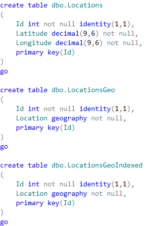
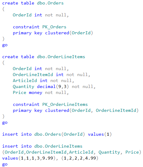
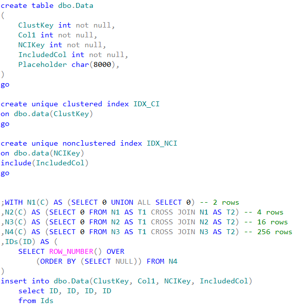
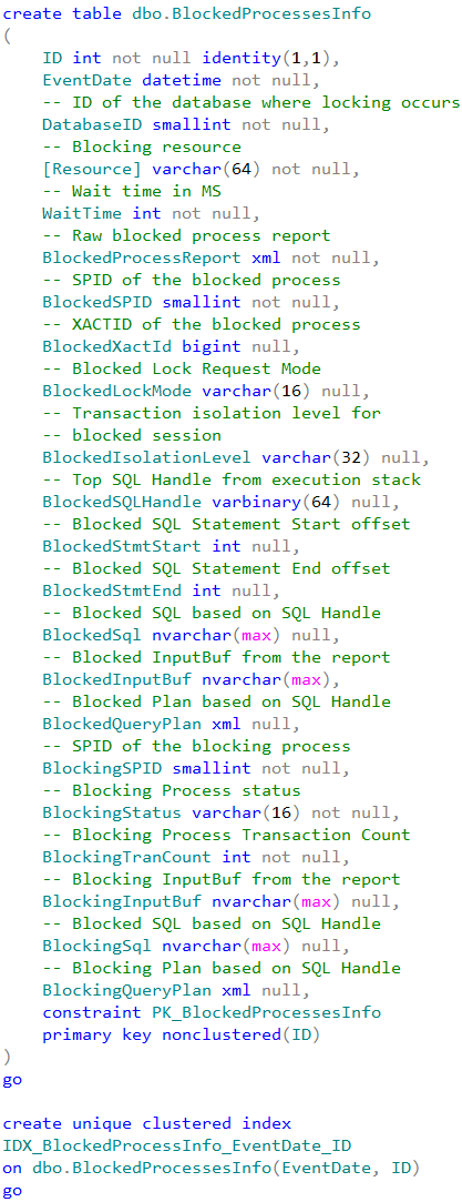
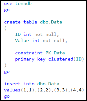
01. Test tables

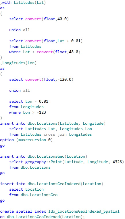
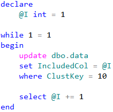
02. Populating test tables with data

The first table dbo.Locations stores the coordinates using decimal(9,6) data type. Two other tables are using geography data type. Finally, the table dbo.LocationsGeoIndexed has Location column indexed with special type of the index called spatial index. Those indexes help improving performance of some operations, for example distance calculation or check if objects are intersecting.

It is worth mentioning that the first table uses decimal(9,6) data type rather than float. This decision saves us six bytes per pair of values and provides the accuracy that exceed the accuracy of commercial-grade GPS receivers.

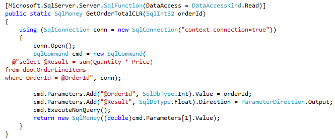
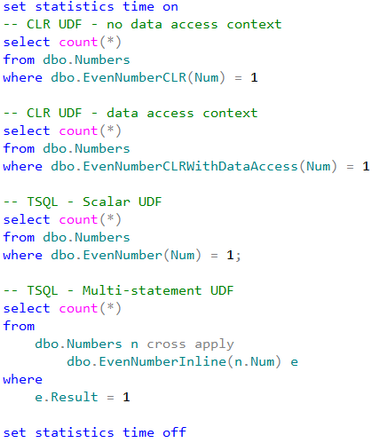
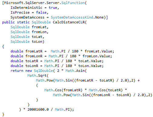
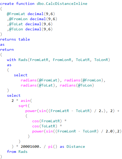
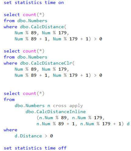
Let’s run the tests that measures performance of the queries that calculate the number of locations within one mile from Seattle City Center. In case of dbo.Locations table, we will use dbo.CalcDistanceCLR function, which we defined earlier. For two other tables we will call spatial method STDistance.

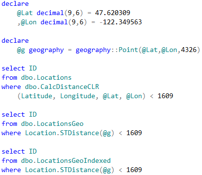
03. Test queries (table-wide lookup)

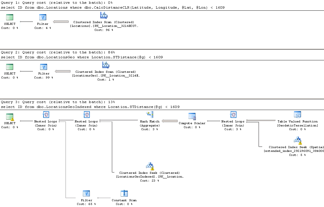
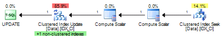
04. Execution plans (table-wide lookup)

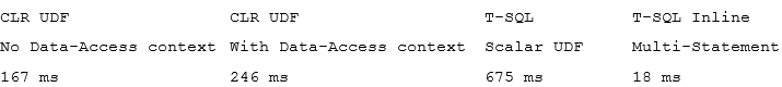
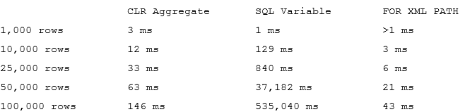
The first and second queries perform clustered index scan and calculate the distance for every row from the table. Last query uses spatial index to lookup such rows. We can see execution times for the queries in the table below.

05. Execution time (Table-wide lookup)

As we see, spatial index greatly benefits the query. It is also worth mentioning, that without the index, performance of CalcDistanceCLR method is better comparing to STDistance.

Although spatial index greatly improves the performance, it has its own limitations. It works in the scope of entire table and all other predicates are evaluated after spatial index operations. That can introduce suboptimal plans in some cases.

As the example, let’s look at the use-case, when we store POI information on company-by-company basis .

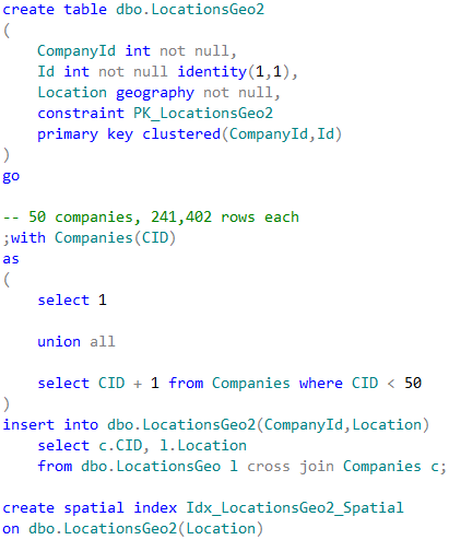
06. Test table creation (company-wide lookup)

In case, when we perform POI lookup for specific company, CompanyId column must be included as the predicate to the queries. SQL Server has two choices how to proceed. The first choice is clustered index seek based on CompanyId value calling STDistance method for every POI that belongs to the company. Another choice is using spatial index, find all POIs within the specified distance regardless of what company they belong and, finally, join it with the clustered index data. Let’s run those queries.

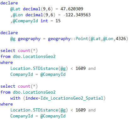
07. Test queries (company-wide lookup)

Neither method is efficient in case when table stores the large amount of data for the large number of companies. Execution plan of the first query utilizing clustered index seek shows that it performed STDistance call 241,402 times – once per every company POI.

08. Execution plan (clustered index seek approach)

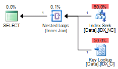
The execution plan for the second query shows that spatial index lookup returned 550 rows – all POI in the area, regardless of what company they belong. SQL Server had to join the rows with the clustered index before evaluating CompanyId predicate.

09. Execution plan (Spatial index approach)

One of the ways to solve such problem called Bounding Box approach. That method allows us to minimize the number of the calculations by filtering out POIs that are outside of the area of interest.
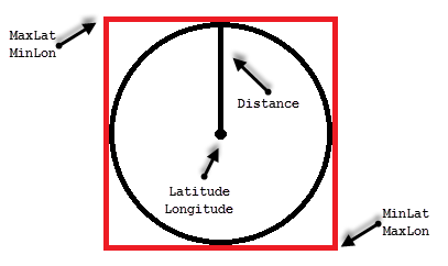
10. Bounding box

All points we need to select residing in the circle with location as the center point and radius specified by the distance. The only points we need to evaluate are residing within the box that inscribes that circle.

We can calculate the coordinates of the corner points of the box, persist it in the table and use regular non-clustered index to pre-filter the data. This would allow us to minimize the number of expensive distance calculations to perform.

Calculation of the bounding box corner points can be done with CLR table-valued function shown below.

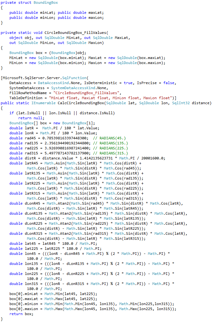
11. Calculating bounding box corner points

Let’s alter our table and add bounding box points. We also need to create non-clustered index to support our query.

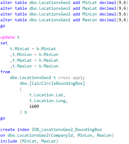
12. Table alteration (adding bounding box corner points)

Now, we can change the query to utilize the bounding box.

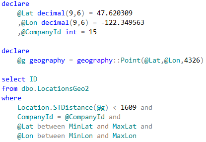
13. Query utilizing bounding box

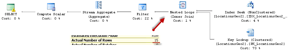
14. Query utilizing bounding box (Execution plan)

As we see, last query calculated the distance 15 times. This is significant improvement comparing to 241,402 calculations from the original query. The execution times are shown below:

15. Execution time (Company-wide lookup)

As we see, bounding box outperforms both – clustered index seek and spatial index lookup. Obviously, it would be the case only when bounding box reduces the number of the calculations to degree that offsets the overhead of non-clustered index seek and key lookup operations. It is also worth mentioning that we do not need spatial index with such approach.

We can use bounding box for the other use-cases. For example, when we are checking if position belongs to the area defined by the polygon. Bounding box corner coordinates should store minimum and maximum latitude/longitude of the polygon corner points. Similarly to the distance calculation, we would filter-out the locations outside of the box before performing expensive spatial method call that validates if point is within the polygon area.

Source code is available for download

CLR: Security considerations

Last time we compared performance of Common Language Runtime (CLR) and T-SQL code in a few different areas. Today, I would like to discuss a few questions related to CLR integration and security. As before, I am not trying to make the point if we should or should not use CLR but rather outline a few things we must take into consideration.

SQL Server has CLR integration disabled by default. Although it would not prevent us from deploying the database with assemblies and CLR objects, we would not be able to call CLR routines until CLR is enabled on the server level. That could lead to the roadblocks for independent software vendors (ISV) who are trying to deploy their systems in Enterprise environments. Database and security administrators often oppose such requirement especially if assemblies require higher than SAFE permission set.

It is worth mentioning that system CLR code is always enabled. We can use system CLR types, such as HierarchyId, Geometry and Geography regardless of the configuration setting.

Second important factor is that we cannot run the code from assemblies with EXTERNAL_ACCESS or UNSAFE permission sets unless they are signed with the key that has such permissions. One of the options to “workaround” it is marking database as TRUSTWORTHY. Although, it violates the best security practices and again, would not necessarily works in the Enterprise environment.

Let’s look at the right way of dealing with such requirement. As the first step we will create the small CLR library with EXTERNAL_ACCESS permission set. You can download the source code if needed.

Let’s create the database and try to register CLR library there. We will get an error as shown below.

01. Registering assembly with EXTERNAL_ACCESS permission set

As we see, we cannot register the assembly as it is. I’m not going to demonstrate the approach with marking database as TRUSTWORTHY and will show how we can sign the assembly.

As the first step, we need to generate the key pair file. We will use sn.exe utility, which is part of Visual Studio and Windows SDK to do that.

02. Generating key pair file with sn.exe

Next, we need to add the generated key file to the CLR project. We can do it in project properties window. Different versions of Visual Studio have slightly different UI there. VS.Net 2012 UI looks like that:

03. Signing the project. VS.Net 2012 UI

When we click Signing button, we will see another popup window where we can specify the key file.

04. Signing the project: VS.Net 2012 UI

After we compiled the signed version of CLR dll we need to create master key in the master database, next create asymmetric key from key pair file, create login from the key and give that login corresponding permission. And after that we will be able to register the assembly.

05. Registering assembly

Now, everything would work just fine.

Finally, CLR objects that accessing the data, break the ownership chaining similarly to dynamic SQL. Let’s create two small test tables and populate it with the data:

07. Ownership chaining: Test tables

Now, let’s create CLR and T-SQL functions that calculate the total amount for specific OrderId provided as the parameter. After that let’s create the views that use those functions

07. Ownership chaining: CLR function

08. Ownership chaining: T-SQL function and views

Finally, let’s create the database user and give him SELECT permissions on both views.

09. Ownership chaining: Creating database user

Now, if user Bob selects data from the view that uses T-SQL function, everything would work fine. Bob has SELECT permission on the view and does not need to have SELECT permissions on the tables as long as owner of the tables and the view is the same because of the ownership chaining.

Although, if user Bob tries to query the view that utilizes CLR function, it would not work.

10. Ownership chaining: CLR breaks ownership chaining

User Bob needs to have SELECT permission on OrderLineItems table in order to CLR function to work

11. Ownership chaining: Permission needs to be granted on the table

That behavior makes permission management more complicated when CLR is involved.

As I mentioned earlier, I am not trying to make the case against CLR. SQL Server Common language runtime integration is very powerful technology. Although we need to be keep in mind performance and security implications, which comes with CLR.

Source code is available for download


CLR vs. T-SQL: Performance considerations

I am pretty sure that all of us read or even participated in quite a few heated discussions about Common Language Runtime (CLR) code in Microsoft SQL Server. Some people state that CLR code works faster than T-SQL, others oppose them. Although, as with the other SQL Server technologies, there is no simple answer to that question. Both technologies are different in nature and should be used for the different tasks. T-SQL is the interpreted language, which is optimized for set-based logic and data access. CLR, on the other hand, produces compiled code that works the best for imperative procedural-style code.

Even with imperative code, we need to decide if we want to implement it in CLR or as the client-side code, perhaps running on the application servers. CLR works within SQL Server process. While, on one hand, it eliminates network traffic and can provide us the best performance due to the “closeness” to the data, CLR adds the load to the SQL Server. It is usually easier and cheaper to scale out application servers rather than upgrading SQL Server box.

There are some cases when we must use CLR code though. For example, let’s think about the queries that performing RegEx evaluations as part of the where clause. It would be inefficient to move such evaluations to the client code and there is no regular expressions support in SQL Server. So CLR is the only choice we have. Although, in the other cases, when procedural-style logic can be moved to the application servers, we should consider such option. Especially when application servers are residing closely to SQL Server and network latency and throughput are not an issue.

Today we will compare performance of the few different areas of CLR and T-SQL. I am not trying to answer the question – “what technology is better”. As usual it fits into “It depends” category. What I want to do is looking how technologies behave in the similar tasks when they can be interchanged.

Before we begin, let’s create the table and populate it with some data.

01. Test table

As the first step, let’s compare the user-defined functions invocation cost. We will use the simple function that accepts the integer value as the parameter and returns 1 in case if that value is even. We can see CLR C# implementation below.

02. Invocation overhead: CLR code

As we can see, there are the attributes specified for each function. Those attributes describes different aspects of UDF behavior and can help Query Optimizer to generate more efficient execution plans. I would recommend specifying them explicitly rather than relying on default values.

One of the attributes – DataAccess – indicates if function performs any data access. When this is the case, SQL Server calls the function in the different context that will allow access to the data. Setting up such context introduces additional overhead during the functional call, which we will see in a few minutes.

T-SQL implementation of those functions would look like that:

03. Invocation overhead: T-SQL code

Let’s measure average execution time for the statements shown below. Obviously, different hardware leads to the different execution time although trends would be the same.

04. Invocation overhead: Test script

Each statement performs clustered index scan of dbo.Numbers table and checks if Num column is even for every row from the table. For CLR and T-SQL scalar user-defined functions, that introduces the actual function call. Inline multi-statement function, on the other hand, performed the calculation inline without function call overhead.

05. Invocation overhead: Avg. Execution Time

As we can see, CLR UDF without data access context performs about four times faster comparing to T-SQL scalar function. Even if establishing data-access context introduces additional overhead and increases execution time, it is still faster than T-SQL scalar UDF implementation.

The key point here though is than in such particular example the best performance could be achieved if we stop using the functions at all rather than converting T-SQL implementation to CLR UDF. Even with CLR UDF, the overhead of the function call is much higher than inline calculations.

Unfortunately, this is not always the case. While we should always think about code refactoring as the option, there are the cases when CLR implementation can outperform inline calculations even with all overhead it introduced. We are talking about mathematical calculations, string manipulations, XML parsing and serialization – to name just a few. Let’s test the performance of the functions that calculate the distance between two points defined by latitude and longitude.

06. Distance Calculation: CLR

07: Calculating Distance: Scalar T-SQL UDF

08. Calculating Distance: Inline function

09. Calculating Distance: Test script

10. Calculating Distance: Execution Time

We can see that CLR UDF runs almost two times faster comparing to inline table-valued functions and more than five times faster comparing to T-SQL scalar UDF. Even with all calling overhead involved.

Now let’s look at the data access performance. The first test compares performance of the separate DML statements from T-SQL and CLR stored procedures. In that test we will create the procedures that calculate the number of the rows in dbo.Numbers table for specific Num interval provided as the parameters. We can see the implementation below

11. Data Access: CLR

12. Data Access: T-SQL

Table below shows the average execution time for stored procedure with the parameters that lead to 50,000 individual SELECT statements. As we can see, data access from CLR code is much less efficient and works about five times slower than data access from T-SQL.

13. Data Access: Individual Statements – execution time

Now let’s compare performance of the row-by-row processing using T-SQL cursor and .Net SqlDataReader class.

14. SqlDataReader vs. cursor: CLR

15. SqlDataReader vs. cursor: T-SQL

16. SqlDataReader vs. Cursor: Execution time

As we can see, SqlDataReader implementation is faster.

Finally, let’s look at the performance of CLR aggregates. We will use standard implementation of the aggregate that concatenates the values into comma-separated string.

17. Building CSV list: Aggregate

As with user-defined functions, it is extremely important to set the attributes that tell Query Optimizer about CLR Aggregate behavior and implementation. This would help to generate more efficient execution plans and prevent incorrect results due to optimization. It is also important to specify MaxByteSize attribute that defines the maximum size of the aggregate output. In our case, we set it to -1 which means that aggregate could hold up to 2GB of data.

Speaking of T-SQL implementation, let’s look at the approach that uses SQL variable to hold intermediate results. That approach implements imperative row-by-row processing under the hood.

As another option let’s use FOR XML PATH technique. It is worth to mention that this technique could introduce different results by replacing XML special characters with character entities. For example, if our values contain < character, it would be replaced with &lt; string.

Our test code would look like that:

18. Building CSV list: T-SQL

When we compare the performance on the different row set sizes, we would see results below

19. Building CSV list: Execution time

As we can see, CLR aggregate has slightly higher startup cost comparing to T-SQL variable approach although it quickly disappears on the larger rowsets. Performance of both: CLR aggregate and FOR XML PATH methods linearly depend on the number of the rows to aggregate while performance of SQL Variable approach degrade exponentially. SQL Server needs to initiate the new instance of the string every time it concatenates the new value and it does not work efficiently especially when it needs to be populated with the large values.

The key point I would like to make with that example is that we always need to look at the options to replace imperative code with declarative set-based logic. While CLR usually outperforms procedural-style T-SQL code, set-based logic could outperform both of them.

While there are some cases when choice between technologies is obvious, there are the cases when it is not clear. Let us think about scalar UDF that needs to perform some data access. Lower invocation cost of CLR function can be mitigated by higher data access cost from there. Similarly, inline mathematical calculations in T-SQL could be slower than in CLR even with all invocation overhead involved. In those cases, we must test different approaches and find the best one which works in that particular case.

Source code is available for download

Next: CLR: Security considerations

Locking in Microsoft SQL Server (Part 18) – Key lookup deadlock

Today I would like us to talk about the special case of the deadlock called key lookup deadlock. This deadlock can happen when multiple sessions are reading and updating the same rows simultaneously. Let us look at the example.

As the first step, let us create the table with the clustered and nonclustered indexes. Nonclustered index has one included column. We are inserting 256 rows there keeping clustered and nonclustered key values the same – from 1 to 256.

Creating the table and populating it with the data

Now let us run two sessions in parallel. In the first session, we are updating the column that included to the nonclustered index using clustered key value in where clause.

Session 1 code

As we can guess, this session will use clustered index seek operation in the execution plan.

Session 1 execution plan

The second session will read the same row using nonclustered key value

Session 2 code

Because Col1 is not part of the nonclustered index, we would have nonclustered index seek and key lookup operations in the execution plan:

Session 2 execution plan

Both statements are running in the loop just to emulate concurrent access to the data. In just a few seconds, we will have the deadlock and session with select would be chosen as the deadlock victim.

Deadlock error

At the first glance, this looks confusing. Both sessions are dealing with the same row. We would expect to have the blocking cases due to exclusive (X) and shared (S) lock incompatibility for the duration of the transaction although we do not expect the deadlock. However, even if we are dealing with the single row, there are two indexes involved.

Let us take a look what locks SQL Server acquires when the table has the multiple indexes. First, let us update the column, which does not belong to nonclustered index, and see what row-level locks will be held.

Updating column that is not part of the nonclustered index

As we see, there is only one exclusive (X) lock on the clustered index. Col1 is not part of nonclustered index and as result, SQL Server does not need to update it and acquire the lock there.

Let us see what happen, if we update the column, which is included to the nonclustered index.

Updating column that is included to the nonclustered index

As we see, now we have two locks in place – one on each index key. And the point here is that we run such update, SQL Server would lock the row in one index first and another index after that. The sequence depends on the execution plan and in our case it would acquire exclusive (X) lock on the clustered index first.

Similarly, our select statement also acquires two shared (S) locks. First, it would lock the row in non-clustered index and then acquire the lock on the clustered index during key lookup operation.

That should give us the idea why we have the deadlock. Both statements are running simultaneously. In the first step, update statement acquires exclusive (X) lock on the row in the clustered index and select statement acquires shared (S) lock on the row in the nonclustered index

Key lookup deadlock: Step 1

After that, update statement is trying to acquire the exclusive (X) lock on the nonclustered index row and being blocked because there is the shared (S) lock held. Same thing happens with select statement, which is trying to acquire shared (S) lock on the clustered index row and being blocked because of the exclusive (X) lock held. Classic deadlock.

Key lookup deadlock: Step 2

To prove that, we can run the statement that shows the current row-level locks immediately after we run our original two sessions. If we are lucky, we can catch the state when both sessions are blocked before deadlock monitor task wakes up and terminate one of the sessions.

Row-level locks in time of the deadlock

There are a few ways that can help to eliminate the deadlock. First option would be eliminating key lookup operation by adding Col1 as included column to the index. In such case, select statement does not need to access the data from the clustered index, which will solve the problem. Unfortunately, that solution increases the size of the nonclustered index key row and introduce additional overhead during data modifications and index maintenance.

Another approach would be switching to optimistic isolation levels where writers do not block readers. While it can help to solve blocking and deadlocking issues, it would also introduce additional tempdb overhead and increases the fragmentation.

Finally, we can refactor the code and separate nonclustered index seek and key lookup operations to two separate selects

Workaround: separating NCI seek and key lookup

Workaround: Execution plan

Both select statements are working on the single index scope and as result would not hold shared (S) locks on the both indexes simultaneously when we are using read committed transaction isolation level. Although, this solution would not work in repeatable read and serializable isolation levels where shared (S) locks held until the end of the transaction.

Source code is available for download

Next: Concurrency model in in-memory OLTP (Hekaton)

Table of content

Locking in Microsoft SQL Server (Part 17) – Implementing Critical Section / Mutexes in T-SQL

Today I’d like us to discuss how we can implement analog of Critical Section (or Mutex) in T-SQL. One of the tasks when it could be beneficial is when we need to prevent the multiple sessions from reading the data simultaneously. As the example let’s think about the system which collects some data and does some kind of post processing after data is inserted.

One of the typical implementation in such architecture would be having the farm of the application servers that do the post processing. We usually need to have more than one server in such scenario for scalability and redundancy reasons. The key problem here is how to prevent the different servers from reading and processing the same data simultaneously. There are a few ways how we can do it. One approach would be using central management server that loads and distributes the data across processing servers. While it could help with the scalability we will need to do something to make that server redundant. Alternatively we can use some sort of distributed cache solution. We could load the data there and every server grabs and processes the data from the cache. That approach could be scalable and work great although distributed cache is not the easy thing to implement. There are the few (expensive) solutions on the market though if you don’t mind to spend money.

There are of course, other possibilities but perhaps the easiest approach from the coding standpoint would be implementing application servers in the stateless manner and do the serialization while reading the data in T-SQL.

Let’s create the table we can use in our exercises and populate it with some data.

A couple things here. First of all, we need to handle the situations when application server crashes and make sure that data would be loaded again after some time by another app server. This is a reason why we are using ReadForProcessing datetime column rather than the simple Boolean flag.

I’d also assume that system wants to read data in FIFO (first in, first out) order as much as possible and after processing is done the data would be moved into another table and deleted from the original RawData table. This is the reason why there is no indexes but clustered primary key. If we need to keep the data in the same table we can do it with additional Boolean flag, for example Processed bit column, although we will need to have another index. Perhaps:

create nonclustered index IDX_RawData_ReadForProcessing
on dbo.RawData(ReadForProcessing)
include(Processed)
where Processed = 0

In addition to the index we also need to assign default value to ReadForProcessing column to avoid ISNULL predicate in the where clause to make it SARGable. We can use some value from the past. 2001-01-01 would work just fine.

In either case, after we read the data for the processing we need to update ReadyForProcessing column with the current (UTC) time. The code itself could look like that:

DataPacket CTE is using ordered clustered index scan. It would stop scanning immediately after read 10 rows (TOP condition). Again, we are assuming that data is moved to another table after the processing so it would be efficient. We are updating the timestamp same time when we read it and saving the package for the client in the temporary table @Result using output clause

The problem here is the race condition when two or more sessions are starting to read and update the data simultaneously. Our update statement would obtain shared (S) locks during select in CTE and after that use update (U) and exclusive (X) locks on the data to be updated.

Obviously different sessions would not be able to update the same rows simultaneously – one session will hold exclusive (X) lock on the row while other sessions would be blocked waiting for shared (S) or update (U) lock. In the first case (shared (S) lock), it’s not a problem – the blocked session will read new (updated) value of ReadForProcessing column as soon as the first session releases the exclusive (X) lock. But in the second case the second session will update (and read) the row the second time. Simplified version of the process is shown below.

At the first step both sessions read the row acquiring and releasing shared (S) locks. Both sessions evaluate the predicate (isnull(ReadForProcessing,’2001-01-01′) < dateadd(minute,-1,GetUtcDate())) and decided to update the row. At this point one of the sessions acquires update(U) and then exclusive (X) lock while other session is blocked.

After the first session releases the exclusive (X) lock, the second session updates the same row.

How can we avoid that? We can create another resource and acquire exclusive lock on that resource before update statement from within the transaction. As we remember, exclusive (X) locks held till the end of transaction, so we will use it as the serialization point. Let’s take a look how it works by creating another table as the lock resource. Now, if we start transaction, we can obtain exclusive table lock. Again, exclusive (X) locks held till the end of transaction, so other sessions would be blocked trying to acquire the lock on the table. As result, execution of our update statement would be serialized.

We can test that approach by running this SP from the multiple sessions simultaneously. There is the artificial delay which we are using during the testing just to make sure that we have enough time to run SP in the different session.

While that approach works, there is another, better way to accomplish the same task. We can use application locks. Basically, application locks are just the “named” locks we can issue. We can use them instead of locking table.

That would lead to the same results.

Application locks are also very useful when we need to implement some code that alters the database schema (for example alter partition function) in the systems that are running under load all the time (24×7). Our DDL statements can issue shared application locks while DDL statements acquire exclusive application locks. This would help to avoid deadlocks related to the lock partitioning. You can see the post about lock partitioning with more details about the problem and implementation.

Although, if we talk about specific task of serialization of the reading process, we don’t need critical section at all. We can use the locking hints instead.

As you can see, there are two locking hints in the select statement. UPDLOCK hint forces SQL Server using update (U) locks rather than shared (S) ones. Update locks are incompatible with each other so multiple sessions would not be able to read the same row. Another hint – READPAST – tells SQL Server to skip the locked rows rather than being blocked. Let’s modify our stored procedure to use that approach.

I’m adding some code to the procedure to emulate race condition. In one session we will run the stored procedure with @UseDelay = 1. In another with @UseDelay = 0. Both of those sessions will start to execute the main update statement roughly at the same time.

This method works even more efficiently than the “critical section” approach. Multiple sessions can read the data in parallel.

Well, I hope that we achieved two goals today. First – we learned how to implement critical section and/or mutexes in T-SQL. But, more importantly, I hope that it taught us that in some cases, the “classic” approach is not the best and we need to think out of the box. Even when this thinking involved the standard functional available in SQL Server.

Source code is available for download

Table of content

Next: Key lookup deadlock


Locking in Microsoft SQL Server (Part 16) – Monitoring Blocked Processes Report with Event Notifications

UPDATE 2018-08-01: New and redesigned version of the code is available here

As we already know it’s very easy to capture blocked process report by using SQL Traces. That method though has a few limitations. First of all, it means we need to have SQL Trace up and running all the time. And SQL Trace, especially the client one, introduces the overhead on SQL Server. Another big problem is that we need to monitor traces on the regular basis. And in case if we had the blocking from within the stored procedures (e.g. session input buffer contains SP reference only), we would need to use sql handles and get the estimate execution plan from the plan cache. Nothing guarantees that plan would be there by the time when we start troubleshooting the blocking problem. Of course, we can set up an alert with SQL Agent and get the notification when blocking
occurs although it would still mean that we have to do our job manually.

As another option we can use Event Notification for BLOCKED_PROCESS_REPORT event. This approach would utilize Service Broker so we would be able to create activation stored procedure and parse blocking report there. Let’s take a look at that.

First of all, we need to decide where to store the data. While we can put the table to the user database, I’d prefer to use separate utility database for the data collection. Let’s do that:

At that point we would have blocked process report events going to dbo.BlockedProcessNotificationQueue service broker queue. Assuming, of course, that we have blocked process threshold option set.

Obviously we do not want to have those messages sitting in the queue – it’s kind of defeating the purpose of having the process automated. What I would like to do at this point is shredding event data and putting it to the table for analysis. Another important factor is that blocked process monitor would generate separate events for the same blocking condition every time it wakes up. For example, if we have blocking process threshold set to 5 seconds, we can get five events until our query times out after 30 seconds. Ideally I’d like to combine those events into the single one to have analysis simplified. So let’s create the table to store the data.

This table stores the information about both – blocked and blocking processes. Although blocking information can be misleading in case if blocking session currently executes the different batch or even waiting for the next batch to be executed – table would store the current state rather than info at the time when blocking occurs. In any cases, from the blocking process standpoint the most interesting attributes are:

  1. Process Status – is it running, sleeping or suspended? If it’s sleeping, it could be the sign that client does not work with transations correctly – either did not commit one of the nested transactions or, perhaps, mixed them with UI activity. Suspended status could be the sign of the blocking chain which is another story
  2. TranCount – if it’s more than one, it would tell us that we have nested transactions and again, perhaps, client does not handle them correctly.

In any case, we will have full report stored and can access it if needed. And of course, we can modify the table and add extra attributes if we want to.

Now it’s the time to put the activation procedure in place. I’m going to cheat a little bit here – click at the link to the source code at the end of the post to see it.

There are two things I’d like to mention though. First one is how we get the query plans.  For the blocked process we are trying to get it from sys.dm_exec_requests first. This is the only bullet-proof way to get the real plan but it would work only if the statement is still blocked when activation SP executes. If this is not the case we are using sys.dm_exec_query_stats DMV. There are a couple challenges though. First, there is the chance that plan would not be there – for example in case of the memory pressure. Alternatively we have the situation when there are multiple plans due recompilation. We are trying to guess the right one by filtering based on the blocking time but that method is not always working. So no guarantees. For the blocking process we are always using sys.dm_exec_query_stats picking up the top (random) plan.

Another thing is how we are looking up if there are other events for the same blocking. Basically stored procedure is trying to match various columns in the merge statement – perhaps even more than needed – but in either case I’d rather have duplicate records than incorrect information.

Last step we need to do is setting up the security. That step is kind of optional in case if we are storing the data in the user database but in our case, when we create the blank database and set up everything under “dbo” user it’s required. When Service Broker activates the stored procedure under that security context (EXECUTE AS OWNER), dbo has enough rights to deal with the database object. But that user also needs to have the rights to query system DMV. As result, we need to create the certificate in the both, EventMonitoring and master databases, create the login from the certificate, grant this login “view server state” and “authenticate server” rights and finally sign the stored procedure with the certificate. Or, perhaps, mark the database as Trustworthy 🙂

And now it’s time for the testing. Let’s create the small table and populate it with a few records.

Next, let’s place exclusive (X) lock on one of the rows in the first session.

In another session let’s introduce the table scan in read committed isolation level.

If we query the service broker queue we would see that there are a few events there. Our queue does not have automatic activation yet.

And finally let’s alter the queue to enable the activation.

Next, let’s query the table.

As we can see, there is the single record in the table now – exactly what we need. This approach is, of course, customizable. You can collect other statistics by changing the implementation. Hope, that script would be the great starting point

Next: Implementing Critical Sections / Mutexes in T-SQL

Table of content


Data Partitioning – Scaling-Out (Part 3: Factors to consider)

Of course, there are plenty other ways to scale-out the system in addition to horizontal partitioning and data sharding. Although in every case we have the same set of factors we need to consider before making the final decision of separating the data between the physical servers. Let’s talk about them today.

Development cost:
Scaling-out would increase development cost. The system becomes more complicated. Often there are additional tiers (application server, data warehouse, etc.) that need to be developed, tested and supported. You also need to have different kind of people in the team – while you can possibly save something by having good rather than exceptional DBA, you’d need to have very good architects and backend developers there. With the current trends when hardware prices are decreasing and development cost is rising, you’d need to consider that aspect very carefully from the beginning.

And of course, there is the question about legacy software. Neither of us want to touch old, often obsolete, code. In some cases we could be lucky and keep everything as is (again, legacy is accessing only operational data and/or we have multiple desktop shortcuts). In other cases we could face very painful and expensive process of refactoring.

Support and maintenance cost:
Well, you’ll have more servers to maintain. And everything depends on how much manual work you are doing. There is not much difference between supporting ten or one hundred servers when everything is automated but it would be completely different story when manual work is involved. PowerShell, policy-based management, data collectors and other tools and technologies – learn them – they are your friends.

Hardware and software cost:
At bare minimum you’ll need to buy OS and SQL Server licenses for each server. A lot of things depend on SQL Server Edition – in some cases scaling out would allow you to use Standard editions on the smaller servers rather than stuck with the Enterprise when you don’t scale out. You can be forced to use Enterprise edition even if you don’t need edition features simply because of 64GB RAM limitation Standard edition has. In some cases you can live with lower end storage too. So you need to carefully plan everything.

And there are the Clouds especially when we talk about SQL Server within VM (Infrastructure As A Service approach). With Clouds the picture changes dramatically. We are paying by the hour – for what we are using. There is no (or minimal) upfront cost for hardware and software. And there are physical limitations in VM configuration (RAM, # of Cores, etc.) as well as slow IO performance. Those limitations could force us to scale out regardless of the cost.

High Availability:
This one is interesting. On the one hand, with multiple servers we have to implement HA strategy multiple times (think about automation again). It introduces additional work but on the other hand gives us better (or, perhaps, different) type of protection. When we use horizontal partitioning, we obviously need to keep our main (operational period) server online if we want the system to be operational. But if the server with historical data is down, it would not affect operational activity. Same with data sharding. If we have one out of ten servers down, only ten percent of the customers would be affected. It still bad but trust me, ten percent of complaining customers are better than one hundred percent.

Of course, everything is in “It depends” category. There is no such thing as strict set of rules when scaling out is appropriate. We need to look at the systems on case by case basis and do our homework all the time.

Data Partitioning – Scaling-Out (Part 2: Data Sharding)

Last time we discussed how to scale-out our system with horizontal partitioning. Another approach that can be helpful is data sharding. With such approach we are creating multiple databases of the same (or very similar) structure and distribute (“shard”) our data between them. The typical use-case for this situation would be the system that collects data from the multiple customers where every customer works with his/her own subset of the data.

When customer logs in to the system, we redirect him/her to specific database. After that customer works within that database only. One of the key differences with horizontal partitioning is that customer-facing UI does not necessarily need to have application server. We still need to implement some sort of “redirector” – the part that knows where customer’s data is located and redirects the application to the right shard database. Although, technically speaking, as soon as it’s done, even regular 2-tier client/server system could work just fine. Don’t take me wrong – I’m not trying to suggest not implementing application server but in some cases legacy systems can work just fine with the minimum modifications.

What are the challenges there? From the customer-facing functional the biggest one is how to deal with the shared data. One of the examples is shared Article list in the point-of-sale system. We need to either replicate the data across all databases or create separate database to store that list. Obviously there are plenty of ways to replicate the data. Perhaps the simplest one would be to use snapshot replication (assuming we can have centralized publisher and articles are generally small). Although it still requires additional efforts to support it. Approach with the separate database introduces its own set of issues. It becomes single point of failure – when this database is down – all shards are down. And of course, there is the question how to access this database from the separate shards. Again, most likely linked servers will be in the game. While it’s not necessarily the big issue performance wise – those shared entities are usually small – it still introduces some overhead from development and
management standpoints.

Second interesting question is the legacy software. Well, again, it’s not necessarily a problem. The database schema remains the same across all shards so legacy software technically can work “As Is”. Assuming, of course, it can connect to and work within the single shard and we don’t mind to have large number of shortcuts on desktop.

Cross-shard database access is challenging. Similarly to horizontal partitioning, we need to design the application server that works across multiple shards. With all development challenges this architecture can be beneficial from performance standpoint – we can query shards in parallel. On the other hand cross-shard access is not always needed. Some of the use-cases (for example, CRM) could be done within the single shard. Others, such as analysis, reporting and accounting, could be implemented in the separate Data Warehouse type database with ETL processes that get the data from the shards. And we rarely need raw transaction data in the data warehouse so size should not be an issue.

One very important question is how to shard the data. In some cases we can have natural criteria – like geographic regions in the picture above. Although we need to be careful when criteria is artificial. Ideally we are looking for uniform data distribution though it could be complicated in some cases. It’s not the good idea to distribute customers data based on ID ranges when, for example, first shard stores IDs between 1 and 1,000; second one – between 1,001 and 2,000 and so on. Old customers (lowest IDs) tend to leave and we will end up with set of underutilized shards. In those cases it’s better to use modulus division: Shard_ID = ID mod Total_Number_Of_Shards.

Another thing to keep in mind is uneven amount of data across for different customers. Let’s think about GPS Tracking as the example when customers are tracking their assets. One customer can have just a few assets, another one hundreds or even thousands of them. Obviously amount of data for those customers would vary greatly. In case, if we have shard servers powerful enough and store large set of the customers per shard, we would be fine. At least should be from statistics standpoint. But it still makes sense to implement some sort of the monitoring solutions to avoid extreme situations.

Next: Scaling-out – Factors to consider

Data Partitioning – Scaling-Out (Part 1: Separating Operational and Historical data)

Before we start talking about Data Partitioning within the same database, I’d like us to discuss a couple methods of partitioning by scaling-out our data and servers. So, first of all, let’s think about the situation when we have all our data in the same database/table.

This is quite general multi-tier client architecture nowadays. Obviously we can have client software (especially legacy one) which is connecting to the database directly.

As we already discussed, almost every system stores two different kinds of data – operational and historical. So what if we do something like that:

In this schema, we keep all operational data and catalog entities in the main database and move historical data to the separate SQL Server(s). We define the linked servers which will allow us to join historical data with catalog entities as well as union the data from the different servers in some cases. Data placement is transparent to the clients which access the data through application server – “the must have” in such architecture. Application server knows how data is stored, queries the data from the multiple databases, merges the streams and returns the final dataset to the clients. Technically speaking, we can even have performance advantages by querying the data in parallel – each database connection could be done from the separate thread.

Legacy software that queries database directly is usually OK too – as long as software does not need access to historical data. Even if historical data is needed, it could be sometimes workarounded by creating distributed partitioned views.

The biggest drawback of this design is additional complexity and overhead introduced by developing the code that combines data from the multiple sources. E.g. application server and, sometimes, database code. Everything would depend on what do we need to do with the data. Some cases are very simple (think about code like that running in the single database/table solution):

With the new multiple servers we will need to open multiple database connections and run those statements against multiple servers:

And finally merge the data for the client. We can even have Customers list cached on application server somewhere and avoid cross-server joins. Simple enough. Although what if we look for something like that – find most expensive orders, page the results and return the second page to the client? (Small disclaimer – it’s not the best way of doing paging. Check this post for more information)

As you can imagine, there are no easy ways to implement it. We need to either write the query that collects the data from the multiple databases via linked servers and sort/page it after that. Alternatively, we can do it on application server side which could lead to the complex code that does not perform well enough. It’s also worth to mention that linked servers could introduce the own set of the issues from both, performance and development standpoints.

The biggest problem I see with such design is that requirements are rarely static – things tend to change. I have this architecture implemented in one of my systems and while things were relatively simple at the beginning, newer requirements led to the huge development overhead. But everything, of course, is system-specific and in “It depends” category. That design has its own purpose and use-cases. And we will talk about them later.

Next: Scaling-Out by Data Sharding

Data Partitioning – When to partition the data

Last week we were discussing why do we want to partition the data. I hope at this point we all agreed that data partitioning could help us with the large table. Which leads to the question – when the table becomes “big enough” for partitioning.

This is kind of theoretical discussion. I heard a lot of different opinions varied from hundreds MBs to TBs. We can spend a lot of time discussing that and will never end up with the right answer. Or, better say, all answers would be the right ones. Obviously your mileage may vary – a lot of things depend on your system, environment and hardware. But my personal take is very simple. If I expect my system to collect large amount of data, the right time (for me) to partition the data is:

Even if Data Partitioning introduces some overhead on development and testing there are two particular reasons why I’d suggest to do that. Most importantly – data partitioning changes execution plans. As result, when you finally implemented it you’d need to re-test entire system. And this could be very expensive and time consuming. Not even mention the possibility of another round of performance tuning. It’s much easier to deal with potential issues during initial development and testing especially when you don’t have a lot of data and impact of sub-optimal execution plans is smaller.

Second reason is that it’s very hard (if even possible) to partition the data keeping the system online. In most part of the cases we are going to deal with exclusive schema modification locks that prevent any access to the table even in read uncommitted transaction isolation level. And if you think how long physical data movement of 100s GBs or TBs of data could take.. Well, you get an idea.

Again, everything depends on the system and requirements. There is no need to spend time and efforts on data partitioning if you don’t expect to have a lot of data. But remember that situation and requirements can change. There is always the possibility that project would be more successful than we expect it to be 🙂

 Next: Scaling Out by separation operational and historical data