Author Archives: Dmitri Korotkevitch

Composite Indexes

Last time we defined when single column index can be used for the index SEEKs. Now let’s talk about composite indexes.

Obviously, the first, and most important question – when composite index can be used for the SEEK operations. Let’s take a look at the example. Let’s create the table with 250,000 rows and create composite index on such table.

Now let’s run a few tests:

As you can see, SQL Server uses index seek each time when predicate on the Column1 (leftmost column) is SARG. The last select where we don’t have the predicate on this column produces the clustered index scan.

So it’s that simple – composite index can be used for the index SEEK as long as predicates on the index leftmost columns are SARG. Well, in real life it’s a little bit more complicated – you should not forget about really small threshold for non-clustered index usage. If SQL Server expects that iterator returns more than a few % of total table rows, index would not be used.

This leads us to quite interesting conclusion. If you have an index on (Column1, Column3), you don’t need to have the separate index on (Column1). Granted, seeks on the second single-column index would be faster because of the smaller row size, but performance benefits you gain in most part of the cases do not worth the price of the index maintenance.

Code can be downloaded from here

Sunday T-SQL Tips: Inserted, Deleted tables and OUTPUT clause (Part 1 – insert/delete/update statements)

During the next a few Sundays I’m planning to talk about one of the under-appreciated constructs in T-SQL – OUTPUT clause. This clause can help you a lot when you need to develop set-based code or convert old cursor-based code into the set operations.

Output clause works together with inserted and deleted system tables. Every developer who wrote at least one DML Trigger familiar with those tables. Those are 2 tables that SQL Server populates and manages automatically. Inserted table contains the new version of the row values. Deleted tables contains the old version of the row values. As you understand inserted table has the data during insert and update operations. Deleted table has the data during update and delete operations.

Let’s see that in the action. First let’s create a table:

Now let’s assume we want to implement the audit trigger. Below is very simple and straightforward approach how we can do that:

Now let’s test the solution.

Below is the XMLs

Anyway, the good and very useful thing that inserted and deleted tables are available not only with the triggers but with insert/update/delete statements. Let’s take a look. First – insert:

As you can see – you have access to generated identity values. You can see that it  works the same way with updates and deletes.

One particularly interesting thing is what happen if statement is rolled back. Let’s populate data to the table again and create the trigger which rollbacks the transaction

Now let’s run the update statement:

As you can see – statement is rolled back – the data has not been changed in the original table but deleted/inserted table were created and populated. Output clause also worked. Such behavior opens the door to the interesting possibilities, for example audit on rollback.

You can download the script from here. Next Sunday we will talk about OUTPUT clause with MERGE statement. This combination is much more powerful than OUTPUT with insert/update/delete.

SQL Saturday 49

I’m going to speak on SQL Saturday #49 this Saturday (10/16/2010) in Orlando. 1 session this time – “Locking and Blocking for Developers”. This is revised version of the presentation I did in Miami – I will put more details to resource waits and bottleneck troubleshooting.

Please stop by if you’re planning to attend.

See you there!

Dmitri

Index Scan and Index Seek

Both operations utilize the indexes. But what is the difference?

Scan operator (on clustered or non-clustered indexes) scans entire index – all data pages and all rows and applies the predicate on every row.

Seek operator “process” only subset of the rows in the index (0..N) – only rows that qualifies.

Assume you have a table:

Now let’s run the select.

As you see, it shows clustered index scan. You can think about that in the following way:

Now let’s create the index on ADate column.

Seek operation does not require to process entire index (rows there are sorted already), so SQL Server finds the first row with ADate = ‘2010-10-01’ and processes the rows until ADate reaches ‘2010-10-02’ and stops.

Obviously index seek operation is much more efficient. But not all predicates are Seekable. What is seekable:
ADate = '2010-10-01'
ADate < '2010-10-02'
ADate between '2010-10-01' and '2010-10-05'
OrderId in (1,3,5)
VarcharField like 'A%'

Basically predicate is seekable if Query Optimizer can map it to the subset of the rows in the index.

Now let’s think about opposite example:

Abs(OrderId) = 1 – Non-seekable predicate. Fortunately you can convert it to: OrderId in (-1, 1)
OrderId + 1 = 10 – Can be converted to: OrderId = 9
DateAdd(day,7,OrderDate) > GetDate() – Can be converted to: OrderDate > DateAdd(day,-7.GetDate())
datepart(year,OrderDate) = 2010 – Can be converted to: OrderDate between '2010-01-01' and '2010-12-31'
VarcharField like '%A%' – here you’re out of luck.

So as you see, functions, calculations on the column makes predicate non-seekable. Avoid that if possible

You can download the code from here

Sunday T-SQL Tip: APPLY operator

One of the new features of SQL 2005 is APPLY operator. Based on books online APPLY is:

The APPLY operator allows you to invoke a table-valued function for each row returned by an outer table expression of a query. The table-valued function acts as the right input and the outer table expression acts as the left input. The right input is evaluated for each row from the left input and the rows produced are combined for the final output. The list of columns produced by the APPLY operator is the set of columns in the left input followed by the list of columns returned by the right input.

A bit confusing if you read it for a first time. Let’s try to clarify it. Think about APPLY the same way as about the JOIN. The difference is that JOIN tables are independent from each other but APPLY is dependent from the left source. There are 2 types of APPLY – CROSS APPLY (think about it as about it as about inner join) and OUTER apply (outer join)

Let’s see it in the example. This will use the orders table created earlier (code can be downloaded from here).

Let’s create the Customers table and populate it with the data

Assuming we want to return the result set that returns 2 most recent orders per customer. Let’s create inline table-valued functions which can do that.

Now let’s write select with cross apply – again think about it as about inner join that joins customer data (source) with 2 rows per customer produced per table-valued function.

Here it is. As you can see – it’s quite simple. What’s interesting about it – you don’t really need to use the function – you can simply put dependent select into the FROM cause. Look below:

You can download the code from here

Covering indexes

We already know the structure of the clustered and non-clustered indexes. We also know what is the main criteria for SQL Server to use non-clustered index.

Today I want to talk about covering indexes technique. Let’s start with the definition.

Covering index for the query is the index that has all required values in the index leaf rows and as result does not require key/bookmark lookup of the actual table data.

Let’s see the example. First of all, let’s create the table and populate it with some data

Now let’s try to run 2 selects – one that return all columns for the customer with id = 100 and second one that returns customerid and orderid only.

As you can see, the first select produces the plan with index seek and key lookup. The second one does not do the key lookup at all. Remember, non-clustered index has the values from the clustered index in the rows so OrderId is there. No needs for the key lookup.

2 Other things I would like to mention. First, you can see that cost of key lookup is 98% of the cost of the first select. Another thing that second select is about 50 times less expensive than the first one.

What should we do if our typical select requires to get a total amount of the orders placed by the customer grouped by date. Obviously we’re filtering (or grouping) by customerid and date in such case. We don’t really need to have amount as additional column in the index because we’re not using it in the predicated. Fortunately SQL Server has a way to add other columns and store it in the index leaf. You can do it with INCLUDE cause of the CREATE INDEX statement.

Below is the picture which show the structure of this index (on some of abstract tables). Click here to open it in the new window.

Let’s check how it works in the example with the orders table:

Plan is index seek, key lookup and next grouping. As you can see it produces 114 logical reads.

Now let’s create the index and run select one more time.

Simple index seek with 2 reads. Great improvement.

Last example I want to show you – let’s try to select max order amount.

As you can see in the first plan – it uses non-clustered index scan. SQL Server cannot use that index for seek operation – but it can scan the index. Because index leaf size is smaller than clustered index row size, it’s more efficient. Look at io statistics

This is one of the easiest optimization techniques you can use in the system – illuminating key lookup with the covering index.

One warning though – extra included columns in the index increase the leaf size, so index will require more pages and be less efficient. So don’t make it extremely wide.

You can download the code from here

Sunday T-SQL Tip: How to generate “Pseudo-identity” values

There are some cases when you don’t want to create physical identity column in the table and want to generate the similar value manually. There are a few methods how to do that. Let’s look at 2 of them.
The first method is the Counters table. Basically you’re creating the table like that:

When you need the new value, you simply get the current one and update it with the new one. It could be wrapped up to the stored procedure like that:

The beauty of this method is the locking – update statement places the exclusive lock on the row so until transaction is active, no other sessions would be able to update the same row. Be careful though with SNAPSHOT isolation level – it would produce an exception during simultaneous access rather than serialize the access.

Let’s test that:

Second method is using identity but from another dummy table:

Let’s see how we can get the single value:

And next – the group of values:

Obviously this method would not protect from the gaps in the values.

You can download the source code from here

When SQL Server uses non-clustered indexes

Last time we took a look at the structure of the indexes. Now let’s talk about index usage in general

Assume you run the query that requires the clustered index scan. Obviously it would require SQL Server to read every data page of the clustered index for the processing. Same time, number of physical reads would be much less than the logical reads. SQL Server uses technique called “Read ahead”. In the nutshells, SQL Server reads up to 64 data pages during the single read operation. So next time SQL Server needs to read the next data page, it most likely would be present in the buffer cache. It still introduces the logical read but obviously would not produce the physical read.

Now let’s think about the operation that scans non non-clustered index. As we know, SQL Server needs to traverse clustered index b-tree for every key/bookmark lookup operation. Even if read-ahead technique would work for the non-clustered index, actual table (clustered index) data could reside anywhere in the data files. So this is basically random IO operation.

Let’s see the example. First of all, let’s create the following table:

Let’s evenly distribute the data for the Name column with the combination of: AAA, AAB, … ZZZ adding 5 rows per each combination and create the non-clustered index on that field

Let’s see some statistics.

As you can see the table has 87880 rows. Clustered index leaf level has 4626 pages and non-clustered index leaf level has 296 pages. Let’s do the tests.

First test. Let’s select rows with Name = ‘ABC’

As you see it returns 5 rows only and leads to 18 logical reads. SQL Server would use non-clustered index for this case.

Second test. Let’s select rows with name starting with ‘AB’

As you see it returns 130 rows and produces 410 logical reads. SQL Server uses non-clustered index. Another thing worth to mention that 99% of the cost of the query is the key lookup.

Next test. Let’s select rows with name starting with ‘A’. Basically it returns 1/26th of the rows which is about 3.8%

As you can see, SQL Server decided to do the clustered index scan which leads to 4644 logical reads.

Let’s run the same select forcing SQL Server to use non-clustered index

As you can see, it produces 10375 logical reads – 2+ times more than clustered index scan. And without any help from read ahead.

So you see – threshold when non-clustered index scan becomes more expensive is really small. SQL Server will not use non-clustered index with key/bookmark lookup in the case if it expects iterator to return more than a few % of the total rows from the table.

Where does it leave us? Make the index highly selective.

Code can be downloaded from here

Sunday T-SQL Tip: Application Locks

There is the set of the tasks when you need to serialize access to some T-SQL code. Assume you have multiple instances of the data processing applications running simultaneously and does not want them to load the same data for the processing. Or you want to perform some bulk operation and want to stop the client from inserting the new data during this period.

Obviously one of the options is to use transactions in serializable isolation level. The problem with that – it could be more restrict than you want to. Supposedly you don’t want to block access to the data but rather introduce something similar to CriticalSection you have with the client development.

Fortunately SQL Server has the set of the stored procedures you can use for such purposes: sp_getapplock and sp_releaseapplock. sp_getapplock allows you to obtain shared or exclusive “user” lock on transaction or session context. If you run this SP in transaction scope, the lock would be released by the end of transaction. Otherwise when session ends.

Let’s see it in action. Let’s run the following statement from 2 different sessions

And here are the results from the both sessions:

As you can see it does the trick.

Update (2013-05-08): This post would provide more details about different methods of serialization available in SQL Server

Indexes structure

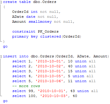
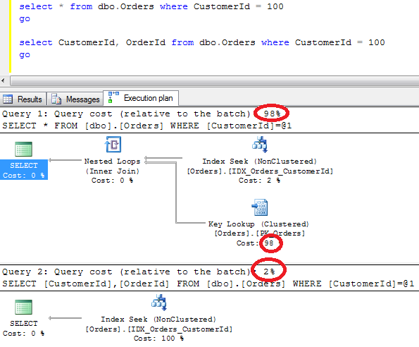
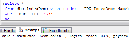
Ok, enough about tables for now. Let’s talk about indexes. As all of us know, there are 2 types of the indexes in SQL Server:

1st – Clustered indexes. This is one index per table and basically specifies the order how data is stored in the table. For example, if the table has the clustered key index on the integer field, it means data will be actually sorted by that integer field. Please don’t be confused – there is still no such thing like default sorting order for the queries – the order of the rows SQL Server returns would depend on the execution plan which could be different than clustered index scan.

SQL Server does not require you to create the clustered indexes – tables without such indexes called heap tables. We will talk about such tables later.

2nd type of the indexes are non-clustered indexes. SQL Server allows to have up to 249 non-clustered indexes per table in SQL 2005 and 999 non-clustered indexes in SQL 2008 (thanks to Chirag for pointing this out). This is “just an index”.

If you think about the book, page number is the clustered index. Alphabetical annotation at the end of the book – is the non-clustered index.

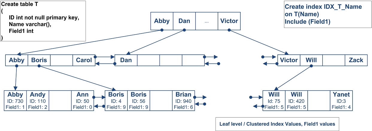
So what exactly is the index? This is B-tree. Let’s see what is that.

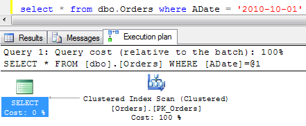
The image above shows a small table with ID as the primary key (and clustered index). As the side note, SQL Server creates clustered index on the primary key field by default.

Leaf level (the bottom one) contains actual table data sorted by ID. As you can see, the data pages are linked into the double-linked list so SQL Server can scan the index in both directions.

Levels above the leaf level called “intermediate levels”. Every index row on those levels points to the separate data pages in the level below. At the top level (root level) there is only one page. There could be several intermedite levels based on the table size. But the top root level of the index always has 1 data page.

So let’s see how it actually works: Assuming you want to select the record with ID = 50. SQL Server start from the root level and find that first row contains ID=1 and the second row contains ID=57. It means that the row with ID=50 would be located on the data page started with ID=1 on the next level of the index. So the next step is analyzing the first data page on the intermediate level which contains IDs from 1 to 50. So SQL Server finds the row with ID=50 and jump on the leaf level page with the actual data.

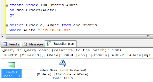
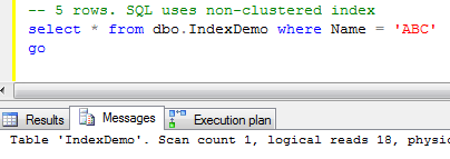
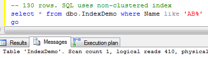
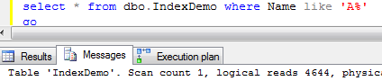
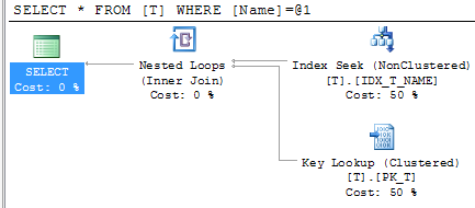
Now let’s look at the non-clustered index. Assuming we have the index by Name field.

The structure of the index is exactly the same with the exception that leaf level does not contain table data but values for the clustered index. It does not really matter if you specify ID in the index definition, it would be there. For the heap tables, leaf level contains actual RID – Row id which consists of FileId:PageNumber:RowNumber. Annotation at the end of the book is a good example. It does not include the actual paragraph from the book but the page # (clustered index)

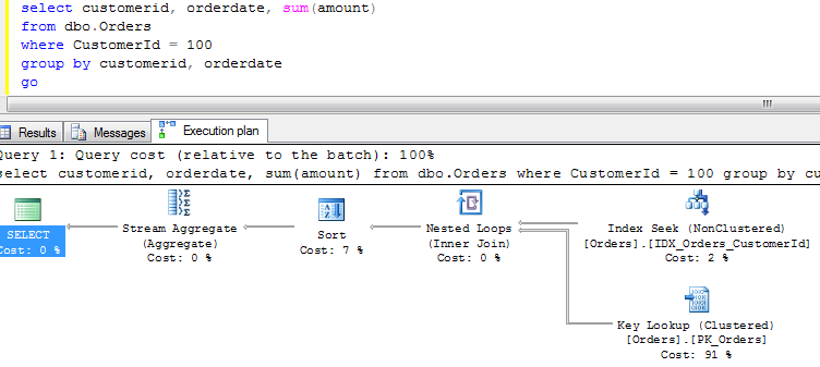
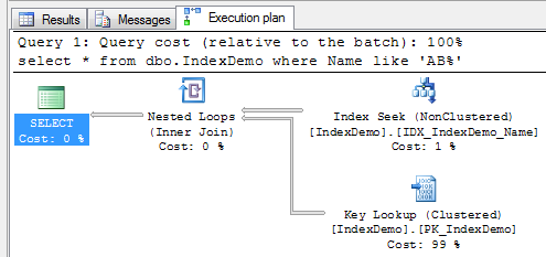
Let’s see how SQL Server works when it uses non-clustered index for the lookups on the tables with clustered index. As you can see, first it needs to find ID of the row(s) and next perform clustered index lookup in order to obtain the actual table data. This operation called “Key lookup” or “Bookmark lookup” on the previous editions of SQL Server.

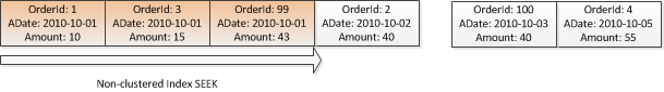
2 things I would like us to remember:
1. Non clustered index has the value of the clustered index on the leaf level
2. As result when SQL Server use non-clustered index for lookup, it needs to traverse clustered index to get the value for the actual data row.

This introduce interesting performance implications we will talk about next time.