Unwinding Table Spools

One of the questions I have often been asked during various SQL Server events is what exactly Table Spool operator does in execution plan. I would try to answer it today.

Spool operators, in the nutshell, are internal in-memory or on-disk caches/temporary tables. SQL Server often uses spools for performance reasons to cache results of complex subexpressions that needs to be used multiple times during query execution.

Let’s look at the example and create the table, which stores some sales information as shown below:

create table dbo.Orders
(
    OrderID int not null,
    CustomerId int not null,
    Total money not null,
    constraint PK_Orders
    primary key clustered(OrderID)
);

;with N1(C) as (select 0 union all select 0) -- 2 rows
,N2(C) as (select 0 from N1 as T1 cross join N1 as T2) -- 4 rows
,N3(C) as (select 0 from N2 as T1 cross join N2 as T2) -- 16 rows
,N4(C) as (select 0 from N3 as T1 cross join N3 as T2) -- 256 rows
,Nums(Num) as (select row_number() over (order by (select null)) from N4)
    insert into dbo.Orders(OrderId, CustomerId, Total)
        select Num, Num % 10 + 1, Num
        from Nums;

Now let’s run the query that returns the list of orders with the information about total amount of sales on per-customer basis.

select OrderId, CustomerID, Total
	,Sum(Total) over(partition by CustomerID) as [Total Customer Sales] 
from dbo.Orders

As you see, in the execution plan below, SQL Server scans the table, sorts the data based on CustomerID order and uses Table Spool operator to cache the results. It allows SQL Server to access the cached data and avoid expensive sorting operation later.

01. Execution Plan with Spool operators

Even though Table Spool operator is shown in the execution plan multiple times, it is essential the same spool/cache. SQL Server builds it the first time and using its data later.

Technically speaking, there are two different logical spool operators – Eager Spool and Lazy Spool. The only difference between them are how data is populated. With Eager Spool, SQL Server fetches all rows as soon as spool is called. With Lazy Spool, SQL Server fetches rows on demand – when they are needed.

SQL Server also uses spools for Halloween Protection when modifying the data. Halloween Protection helps to avoid situations when data modifications affect what data need to be updated. The classic example of such situation is shown below. Without Halloween Protection, insert statement would fall into infinitive loop, reading rows it has been inserting.

create table dbo.HalloweenProtection
(
	Id int not null identity(1,1),
	Data int not null
);

insert into dbo.HalloweenProtection(Data)
	select Data from dbo.HalloweenProtection;

As you can see in the execution plan of insert statement, SQL Server uses Table Spool operator to cache the data from table as of before insert starts to avoid infinitive loop during execution.

02. Halloween Protection and Table Spools.

Halloween Protection has very interesting side-effect when we are talking about multi-statement user-defined functions (both, scalars and table-valued). Using multi-statement functions is bad practice by itself, however creating them without SCHEMABINDING option is even worse. That option forces SQL Server to analyze if user-defined function performs data access and avoid extra Halloween Protection-related Spool operators in the execution plan.

Let’s see the example and create two user-defined functions and using them in where clause of update statements.

create function dbo.ShouldUpdateData(@Id int)
returns bit
as
begin
	return (1)
end
go

create function dbo.ShouldUpdateDataSchemaBound(@Id int)
returns bit
with schemabinding
as
begin
	return (1)
end
go

update dbo.HalloweenProtection
set Data = 0
where dbo.ShouldUpdateData(ID) = 1;

update dbo.HalloweenProtection
set Data = 0
where dbo.ShouldUpdateDataSchemaBound(ID) = 1;

Neither of functions access the data and therefore can introduce Halloween effect. However, SQL Server does not know that in case of non-schema bound function and add Spool operator to execution plan as shown below.

03. Execution Plans for user-defined functions

Bottom line – you should always make functions schema-bound when you create them.

Spool temporary tables are usually referenced as worktables in I/O statistics for the queries. You should analyze table spool-related reads during query performance tuning. While spools can improve performance of the queries, there is the overhead introduced by unnecessary spools. You can often remove them by creating appropriate indexes on the tables.

SQL Server Storage Engine: Heap Tables

Heap tables are tables without a clustered index. The data in heap tables is unsorted.  SQL Server does not guarantee nor maintain any sorting order of the data in the heap tables.
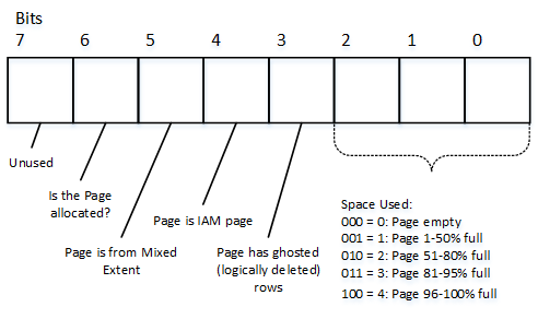
When we insert data into heap tables, SQL Server tries to fill pages as much as possible, although it does not analyze the actual free space available on a page. It uses the Page Free Space (PFS) allocation map instead. SQL Server errs on the side of caution, and it uses the low value from the PFS free space percentage tier during the estimation.

For example, if a data page stores 4,100 bytes of data, and, as result, has 3,960 bytes of free space available, PFS would indicate that the page is 51-80 percent full. SQL Server would not put a new row to the page if its size exceeds 20 percent (8,060 bytes * 0.2 = 1,612 bytes) of the page size.

Let’s look at the example and create the table with the code shown below.

create table dbo.Heap(Val varchar(8000) not null);

;with CTE(ID,Val) as 
(
    select 1, replicate('0',4089)
    union all
    select ID + 1, Val from CTE where ID < 20 
) 
insert into dbo.Heap(Val)
   select Val from CTE;

select page_count, avg_record_size_in_bytes, avg_page_space_used_in_percent
from sys.dm_db_index_physical_stats(db_id(),object_id(N'dbo.Heap'),0,null,'DETAILED');

01. Page Count after initial insert

At this point, the table stores 20 rows of 4,100 bytes each. SQL Server allocates 20 data pages—one page per row—with 3,960 bytes available. PFS would indicate that pages are 51-80 percent full.

As the next step, let’s inserts the small 111-byte row, which is about 1.4 percent of the page size. As a result, SQL Server knows that the row would fit into one of the existing pages (they all have at least 20 percent of free space available), and a new page should not be allocated.

insert into dbo.Heap(Val) values(replicate('1',100));

select page_count, avg_record_size_in_bytes, avg_page_space_used_in_percent 
from sys.dm_db_index_physical_stats(db_id(),object_id(N'dbo.Heap'),0,null,'DETAILED');

02. Page Count after insertion of small row

Lastly, the third insert statement needs 2,011 bytes for the row, which is about 25 percent of the page size. SQL Server does not know if any of the existing pages have enough free space to accommodate the row and, as a result, allocates the new page. You can see that SQL Server does not access existing pages by checking the actual free space and uses PFS data for the estimation.

insert into dbo.Heap(Val) values(replicate('2',2000));

select page_count, avg_record_size_in_bytes, avg_page_space_used_in_percent 
from sys.dm_db_index_physical_stats(db_id(),object_id(N'dbo.Heap'),0,null,'DETAILED');

03. Page Count after insertion of large row

That behavior leads to the situation where SQL Server unnecessarily allocates new data pages, leaving large amount of free space unused. It is not always a problem when the size of rows vary—in those cases, SQL Server eventually fills empty spaces with the smaller rows. However, especially in cases when all rows are relatively large, you can end up with large amounts of wasted space.

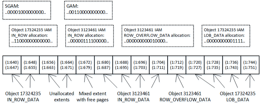
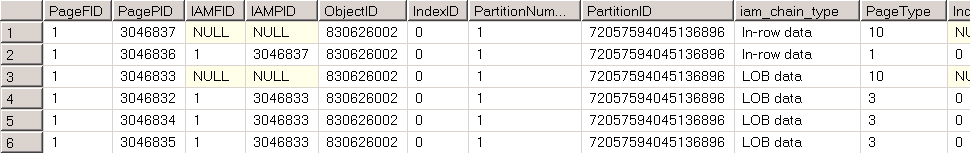
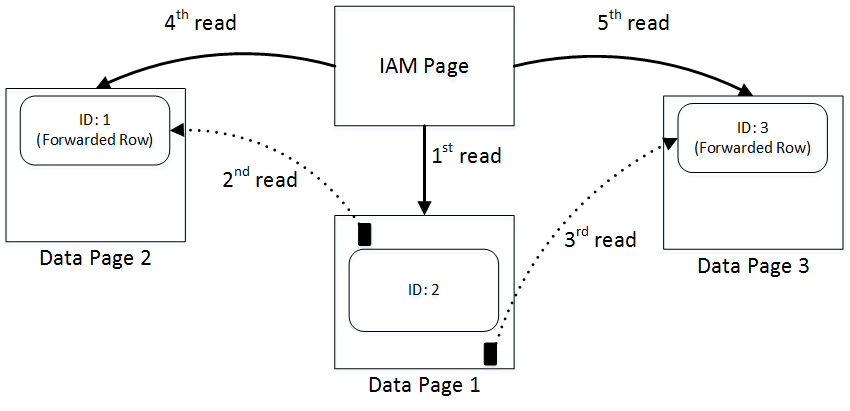
When selecting data from the heap table, SQL Server uses as Index Allocation Map (IAM) to find the pages and extents that need to be scanned. It analyzes what extents belong to the table and processes them based on their allocation order rather than on the order in which the data was inserted. You can see it in figure below.
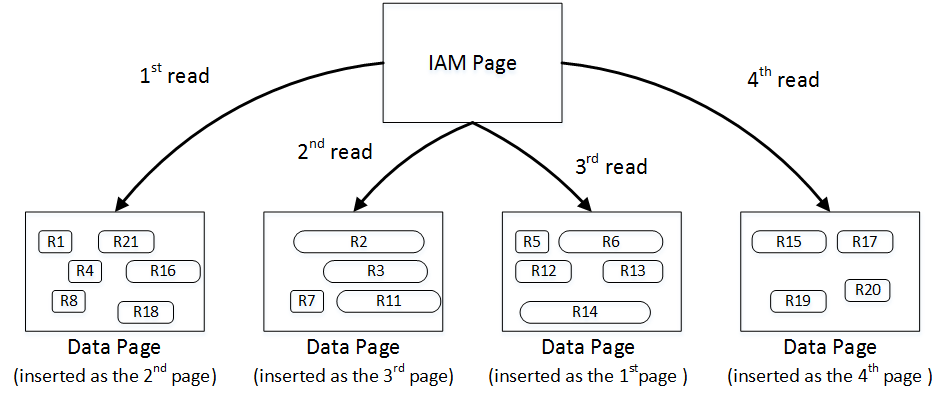
04. IAM Scan

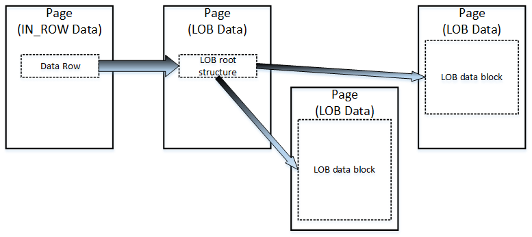
When you update the row in the heap table, SQL Server tries to accommodate it on the same page. If there is no free space available, SQL Server moves the new version of the row to another page and replaces the old row with a special 16-byte row called a forwarding pointer. The new version of the row is called forwarded row.

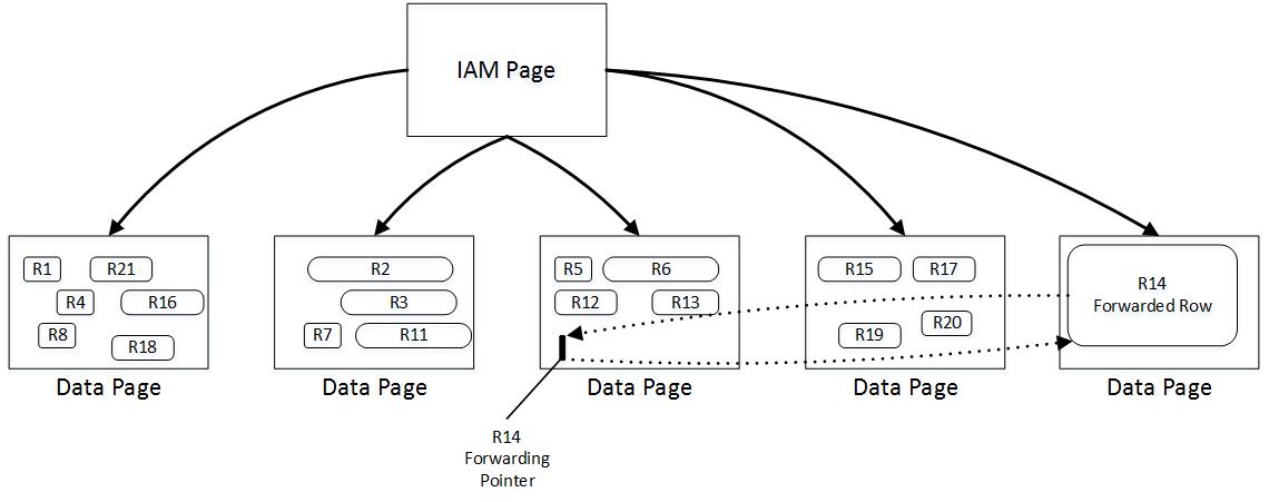
05. Forwarding Pointers

There are two main reasons why forwarding pointers are used. First, they prevent updates of nonclustered index keys, which referencing the row.

In addition, forwarding pointers helps minimize the number of duplicated reads – the situation when a single row is read multiple times during the table scan. As the example, let’s look at figure above and assume that SQL Server scans the pages in left-to-right order. Next, let’s assume that the row in page 3 was modified after the page was read at the time when SQL Server reads page 4. The new version of the row would be moved to page 5, which has yet to be processed. Without forwarding pointers, SQL Server would not know that the old version of the row had already been read, and it would read it again during the page 5 scan. With forwarding pointers, SQL Server would ignore the forwarded rows.

Forwarding pointers help minimize duplicated reads at cost of additional read operations. SQL Server follows the forwarding pointers and reads the new versions of the rows at the time it encounters them. That behavior can introduce an excessive number of I/O operations.

Let’s create the table and insert three rows there.

create table dbo.ForwardingPointers
(
   ID int not null,
   Val varchar(8000) null
);

insert into dbo.ForwardingPointers(ID,Val)
values
   (1,null),
   (2,replicate('2',7800)),
   (3,null);

select page_count, avg_record_size_in_bytes, avg_page_space_used_in_percent, forwarded_record_count
from sys.dm_db_index_physical_stats(db_id(),object_id(N'dbo.ForwardingPointers'),0,null,'DETAILED');

set statistics io on
select count(*) as [RowCnt] from dbo.ForwardingPointers
set statistics io off

You can see results below

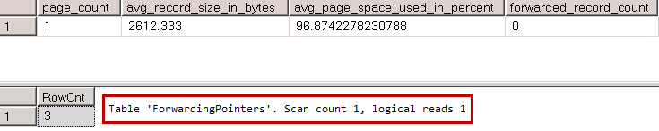
06. Forwarding Pointers: I/O without forwarding pointers

All three rows fit into the single page, and SQL Server needs to read just that page when it scans the table.

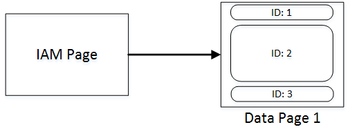
07. Page Layout without Forwarding Pointers

Let’s update two of the table rows and increase their size. The new version of the rows would not fit into the page anymore, which introduces the allocation of the two new pages and two forwarding pointers.

update dbo.ForwardingPointers set Val = replicate('1',5000) where ID = 1;
update dbo.ForwardingPointers set Val = replicate('3',5000) where ID = 3;

select page_count, avg_record_size_in_bytes, avg_page_space_used_in_percent, forwarded_record_count
from sys.dm_db_index_physical_stats(db_id(),object_id(N'dbo.ForwardingPointers'),0,null,'DETAILED');

set statistics io on
select count(*) as [RowCnt] from dbo.ForwardingPointers
set statistics io off

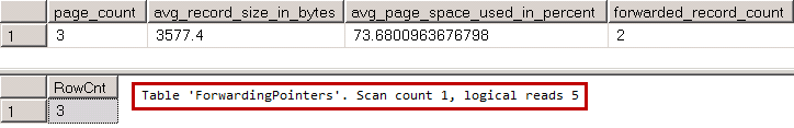
08. Forwarding Pointers: I/O with Forwarding Pointers

When SQL Server reads the forwarding pointer rows from page 1, it follows them and reads pages 2 and 3 immediately thereafter. After that, SQL Server reads those pages one more time during the regular IAM scan process. As a result, we have five read operations, even though our table has just three data pages.

09. Page Layout and I/O with Forwarding Pointers

It does not look as bad in case of the small table. Let’s look at the same issue in case, when table has more rows. Let’s insert 65,536 rows to our table.

truncate table dbo.ForwardingPointers
go

;with N1(C) as (select 0 UNION ALL select 0) -- 2 rows
,N2(C) as (select 0 from N1 as T1 cross join N1 as T2) -- 4 rows
,N3(C) as (select 0 from N2 as T1 cross join N2 as T2) -- 16 rows
,N4(C) as (select 0 from N3 as T1 cross join N3 as T2) -- 256 rows
,N5(C) as (select 0 from N4 as T1 cross join N4 as T2) -- 65,536 rows
,IDs(ID) as (select row_number() over (order by (select NULL)) from N5)
insert into dbo.ForwardingPointers(ID)
	select ID from IDs;

select page_count, avg_record_size_in_bytes, avg_page_space_used_in_percent, forwarded_record_count
from sys.dm_db_index_physical_stats(db_id(),object_id(N'dbo.ForwardingPointers'),0,null,'DETAILED');

set statistics io on
select count(*) as [RowCnt] from dbo.ForwardingPointers
set statistics io off

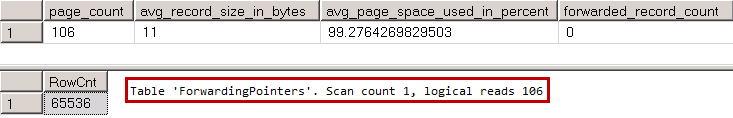
10. Large table: I/O without Forwarding Pointers

As you see, there are 106 pages in the table and as result, SQL Server performs 106 reads during IAM scan. Let’s update our table and introduce forwarding pointers.

update dbo.ForwardingPointers set Val = replicate('a',500);

select page_count, avg_record_size_in_bytes, avg_page_space_used_in_percent, forwarded_record_count
from sys.dm_db_index_physical_stats(db_id(),object_id(N'dbo.ForwardingPointers'),0,null,'DETAILED');

set statistics io on
select count(*) as [RowCnt] from dbo.ForwardingPointers
set statistics io off

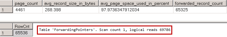
11. Large Table: I/O with Forwarding Pointers

Now our table has 4,461 pages however it requires almost 70 thousand reads to perform a scan. As you see, the large number of the forwarding pointers leads to extra I/O operations and significantly reduces the performance of the queries accessing the data.

When the size of the forwarded row is reduced by another update and the data page with forwarding pointer has enough space to accommodate updated version of the row, SQL Server might move it back to original data page and remove the forwarding pointer. Nevertheless, the only reliable way to get rid of the all forwarding pointers is by rebuilding the heap table. You can do that by using an ALTER TABLE REBUILD statement or by creating and dropping a clustered index on the table.

Heap tables can be useful in staging environment where you want to import a large amount of data into the system as fast as possible. Inserting data into heap tables can often be faster than inserting it into tables with clustered indexes. Nevertheless, during a regular workload, tables with clustered indexes usually outperform heap tables due to their suboptimal space control and forwarding pointers.

Table of content

SQL Server Storage Engine: Allocation Maps

SQL Server logically groups eight pages into 64KB units called extents. There are two types of extents available: Mixed extents store data that belongs to different objects. Uniform extents store the data for the same object.

When a new object is created, SQL Server stores first eight object pages in mixed extents. After that, all subsequent space allocation for that object is done with uniform extents.

SQL Server uses special kind of pages, called Allocation Maps, to track extent and page usage in a file. There are several different types of allocation maps pages in SQL Server.

Global Allocation Map (GAM) pages track if extents have been allocated by any objects. The data is represented as bitmaps where each bit indicates the allocation status of an extent. Zero bits indicate that the corresponding extents are in use. The bits with a value of one indicate that the corresponding extents are free. Every GAM page covers about 64,000 extents, or almost 4GB of data. This means that every database file has one GAM page for about 4GB of file size.

Shared Global Allocation Map (SGAM) pages track information about mixed extents. Similar to GAM pages, it is a bitmap with one bit per extent. The bit has a value of one if the corresponding extent is a mixed extent and has at least one free page available. Otherwise, the bit is set to zero. Like a GAM page, SGAM page tracks about 64,000 extents, or almost 4GB of data.

SQL Server can determine the allocation status of the extent by looking at the corresponding bits in GAM and SGAM pages. Figure below shows the possible combinations of the bits.

01. GAM and SGAM bit statuses

When SQL Server needs to allocate a new uniform extent, it can use any extent where a bit in the GAM page has the value of one. When SQL Server needs to find a page in a mixed extent, it searches both allocation maps looking for the extent with a bit value of one in a SGAM page and the corresponding zero bit in a GAM page. If there are no such extents available, SQL Server allocates the new free extent based on the GAM page, and it sets the corresponding bit to one in the SGAM page.

Every database file has its own chain of GAM and SGAM pages. The first GAM page is always the third page in the data file (page number 2). The first SGAM page is always the fourth page in the data file (page number 3). The next GAM and SGAM pages appear every 511,230 pages in the data files which allows SQL Server to navigate through them quickly when needed.

SQL Server tracks the pages and extents used by the different types of pages (in-row, row-overflow, and LOB pages), that belong to the object with another set of the allocation map pages, called Index Allocation Map (IAM). Every table/index has its own set of IAM pages, which are combined into separate linked lists called IAM chains. Each IAM chain covers its own allocation unit – IN_ROW_DATA, ROW_OVERFLOW_DATA, and LOB_DATA.

Each IAM page in the chain covers a particular GAM interval and represents the bitmap where each bit indicates if a corresponding extent stores the data that belongs to a particular allocation unit for a particular object. In addition, the first IAM page for the object stores the actual page addresses for the first eight object pages, which are stored in mixed extents.

The figure below shows a simplified version of the allocation map pages bitmaps.

02. Allocation maps

Partitioned tables and indexes have separate IAM chains for every partition. In fact, you can consider non-partitioned table as the partitioned with just a single partition.

There is another type of allocation map page called Page Free Space (PFS). Despite the name, PFS pages track a few different things. We can call PFS as a byte-mask, where every byte stores information about a specific page, as shown below.

03. PFS byte structure

The first three bits in the byte indicate the percent of used space on the page. SQL Server tracks the used space for row-overflow and LOB data, as well as for in-row data in the heap tables. These are the only cases when amount of free space on the page matters.

When you delete a data row from the table, SQL Server does not remove it from the data page but rather marks the row as deleted. Bit 4 indicates if the page has logically deleted (ghosted) rows.

Bit 5 indicates if the page is an IAM page. Bit 6 indicates whether or not the page is in the mixed extent. Finally, bit 7 indicates if the page is allocated.

Every PFS page tracks 8,088 pages or about 64MB of data space. It is always the second page (page 1) in the file and every 8,088 pages thereafter.

There are two more types of allocation map pages. The seventh page (page 6) in the file is called a Differential Changed Map (DCM). These pages keep track of extents that have been modified since the last FULL database backup. SQL Server uses DCM pages when it performs DIFFERENTIAL backups.

The last allocation map is called Bulk Changed Map (BCM). It is eighth page (page 7) in the file, and it indicates what extents have been modified in minimally-logged operations since the last transaction log backup. BCM pages are used only with a BULK_LOGGED database recovery model.

Both, DCM and BCM pages are the bitmasks that cover 511,230 pages in the data file.

Next: HEAP tables

Table of Content

SQL Server Storage Engine: LOB Storage

As you already know, the fixed-length data and the internal attributes of a row must fit into a single page. Fortunately, SQL Server can store the variable-length data on different data pages. There are two different ways to store the data, depending on the data type and length.

ROW_OVERFLOW storage

SQL Server stores variable-length column data, which does not exceed 8,000 bytes, on special pages called ROW_OVERFLOW pages. Let’s create a table and populate it with the data shown in listing below.

create table dbo.RowOverflow 
( 
    ID int not null, 
    Col1 varchar(8000) null, 
    Col2 varchar(8000) null 
);

insert into dbo.RowOverflow(ID, Col1, Col2) 
values (1,replicate('a',8000),replicate('b',8000));

SQL Server creates the table and inserts the data row without any errors, even though the data row size exceeds 8,060 bytes. Let’s look at the table page allocation using the DBCC IND command.

DBCC IND('SqlServerInternals','dbo.RowOverflow',-1)


01. ROW_OVERFLOW data: DBCC IND results

Now you can see two different sets of IAM and data pages. The data page with PageType=3 represents the data page that stores ROW_OVERFLOW data.

Let’s look at data page 214647, which is the in-row data page that stores main row data. The partial output of the DBCC PAGE command for the page (1:214647) is shown below.

Slot 0 Offset 0x60 Length 8041

Record Type = PRIMARY_RECORD Record Attributes = NULL_BITMAP VARIABLE_COLUMNS
Record Size = 8041 
Memory Dump @0x000000000FB7A060
0000000000000000:30000800 01000000 03000002 00511f69 9f616161 0............Q.iŸaaa
0000000000000014:61616161 61616161 61616161 61616161 61616161 aaaaaaaaaaaaaaaaaaaa
0000000000000028:61616161 61616161 61616161 61616161 61616161 aaaaaaaaaaaaaaaaaaaa
000000000000003C:61616161 61616161 61616161 61616161 61616161 aaaaaaaaaaaaaaaaaaaa
0000000000000050:61616161 61616161 61616161 61616161 61616161 aaaaaaaaaaaaaaaaaaaa
<Skipped>
0000000000001F2C:61616161 61616161 61616161 61616161 61616161 aaaaaaaaaaaaaaaaaaaa
0000000000001F40:61616161 61616161 61616161 61616161 61020000 aaaaaaaaaaaaaaaaa...
0000000000001F54:00010000 00290000 00401f00 00754603 00010000 .....)...@...uF.....
0000000000001F68:00

As you see, SQL Server stores Col1 data in-row. Col2 data, however, has been replaced with a 24-byte value. The first 16 bytes are used to store off-row storage metadata attributes, such as type, length of the data, and a few other attributes. The last 8 bytes is the actual pointer to the row on the row-overflow page, which is the file, page, and slot number. Figure below shows this in detail. Remember that all information is stored in byte-swapped order.

02. ROW_OVERFLOW page pointer

As you see, the slot number is 0, file number is 1, and page number is the hexadecimal value 0x00034675, which is decimal 214645. The page number matches the DBCC IND results shown earlier in the post.

The partial output of the DBCC PAGE command for the page (1:214645) is shown below.

Blob row at: Page (1:214645) Slot 0 Length: 8014 Type: 3 (DATA)
Blob Id:2686976

0000000008E0A06E: 62626262 62626262 62626262 62626262 bbbbbbbbbbbbbbbb
0000000008E0A07E: 62626262 62626262 62626262 62626262 bbbbbbbbbbbbbbbb
0000000008E0A08E: 62626262 62626262 62626262 62626262 bbbbbbbbbbbbbbbb

Col2 data is stored in the first slot on the page.

LOB Storage

For the text, ntext, or image columns, SQL Server stores the data off-row by default. It uses another kind of page called LOB data pages. You can control this behavior by using the “text in row” table option. For example, exec sp_table_option dbo.MyTable, ‘text in row’, 200 forces SQL Server to store LOB data less or equal to 200 bytes in-row. LOB data greater than 200 bytes would be stored in LOB pages.

The logical LOB data structure is shown below.

03: LOB data structure

Like ROW_OVERFLOW data, there is a pointer to another piece of information called the LOB root structure, which contains a set of the pointers to other data pages/rows. When LOB data is less than 32 KB and can fit into five data pages, the LOB root structure contains the pointers to the actual chunks of LOB data. Otherwise, the LOB tree starts to include an additional, intermediate level of pointers, similar to the index B-Tree.

Let’s create the table and insert one row of data there.

create table dbo.TextData
(
    ID int not null,
    Col1 text null
);

insert into dbo.TextData(ID, Col1) 
values (1, replicate(convert(varchar(max),'a'),16000));

The page allocation for the table is shown below.

04. LOB data: DBCC IND results

As you see, the table has one data page for in-row data and three data pages for LOB data. I am not going to examine the structure of the data row for in-row allocation; it is similar to the ROW_OVERFLOW allocation. However, with the LOB allocation, it stores less metadata information in the pointer and uses 16 bytes rather than the 24 bytes required by the ROW_OVERFLOW pointer.

The result of DBCC PAGE command for the page that stores the LOB root structure is shown below.

Blob row at: Page (1:3046835) Slot 0 Length: 84 Type: 5 (LARGE_ROOT_YUKON)
Blob Id: 131661824 Level: 0 MaxLinks: 5 CurLinks: 2
Child 0 at Page (1:3046834) Slot 0 Size: 8040 Offset: 8040 
Child 1 at Page (1:3046832) Slot 0 Size: 7960 Offset: 16000

As you see, there are two pointers to the other pages with LOB data blocks, which are similar to the blob data stored in ROW_OVERFLOW pages.

The format, in which SQL Server stores the data from the (MAX) columns, such as varchar(max), nvarchar(max), and varbinary(max), depends on the actual data size. SQL Server stores it in-row when possible. When in-row allocation is impossible, and data size is less or equal to 8,000 bytes, it stored as ROW_OVERFLOW data. The data that exceeds 8,000 bytes is stored as LOB data.

It is also worth mentioning that SQL Server always stores rows that fit into a single page using in-row allocations. When a page does not have enough free space to accommodate a row, SQL Server allocates a new page and places the row there rather than placing it on the half-full page and moving some of the data to ROW_OVERFLOW pages.

SELECT * and I/O

There are plenty of reasons why selecting all columns from a table with the select * operator is not a good idea. It increases network traffic by transmitting columns that the client application does not need. It also makes query performance tuning more complicated, and it introduces side effects when the table schema changes.

It is recommended that you avoid such a pattern and explicitly specify the list of columns needed by the client application. This is especially important with ROW_OVERFLOW and LOB storage, when one row can have data stored in multiple data pages. SQL Server needs to read all of those pages, which can significantly decrease the performance of queries.

As an example, let’s assume that we have table dbo.Employees with one column storing employee pictures.

create table dbo.Employees
(
    EmployeeId int not null,
    Name varchar(128) not null,
    Picture varbinary(max) null
);

;WITH N1(C) AS (SELECT 0 UNION ALL SELECT 0) -- 2 rows
,N2(C) AS (SELECT 0 FROM N1 AS T1 CROSS JOIN N1 AS T2) -- 4 rows
,N3(C) AS (SELECT 0 FROM N2 AS T1 CROSS JOIN N2 AS T2) -- 16 rows
,N4(C) AS (SELECT 0 FROM N3 AS T1 CROSS JOIN N3 AS T2) -- 256 rows
,N5(C) AS (SELECT 0 FROM N4 AS T1 CROSS JOIN N2 AS T2) -- 1,024 rows
,IDs(ID) AS (SELECT ROW_NUMBER() OVER (ORDER BY (SELECT NULL)) FROM N5)
insert into dbo.Employees(EmployeeId, Name, Picture)
    select   
        ID
        ,'Employee ' + convert(varchar(5),ID)
        ,convert(varbinary(max),replicate(convert(varchar(max),'a'),120000))
    from Ids;

The table has 1,024 rows with binary data of 120,000 bytes. Let’s assume that we have code in the client application that needs the EmployeeId and Name to populate a drop-down box. If a developer is not careful, he can write a select statement using the select * pattern, even though a picture is not needed for this particular use-case.

Let’s compare the performance of two selects; one selecting all data columns and another that selects only EmployeeId and Name

set statistics io on
set statistics time on

select * from dbo.Employees;
select EmployeeId, Name from dbo.Employees;

set statistics io off
set statistics time off
Results:
select EmployeeId, Name from dbo.Employee: 
Number of reads: 7;  Execution time (ms): 2

select * from dbo.Employee
Number of reads: 90,895; Execution time (ms): 343

As you see, the first select, which reads the LOB data and transmits it to the client, is a few orders of magnitude slower than the second select.

One case where this becomes extremely important is with client applications, which use Object Relational Mapping (ORM) frameworks. Developers tend to reuse the same entity objects in different parts of an application. As a result, an application may load all attributes/columns even though it does not need all of them in many cases.

It is better to define different entities with a minimum set of required attributes on an individual use-case basis. In our example, it would work best to create separate entities/classes, such as EmployeeList and EmployeeProperties. An EmployeeList entity would have two attributes: EmployeeId and Name. EmployeeProperties would include a Picture attribute in addition to the two mentioned.

This approach can significantly improve the performance of systems.

Next: Allocation Maps

Table of Content

SQL Server Storage Engine: Data Pages and Data Rows

The space in the database divided into logical 8KB pages. Those pages are continuously numbered starting with zero and can be referenced by specifying a file ID and a page number. The page numbering is always continuous – when SQL Server grows the database file, the new pages would have the numbers starting from the last highest page number in the file plus one. Similar, when SQL Server shrinks the file, it removes the highest number pages from the file.

Let’s look at the structure of a data page. All images are clickable.

01. Data Page Structure

96-bytes page header contains the various information about a page , such as the  object page belongs; number of rows and amount of free space available on the page; links to the previous and next pages if the page is in an index page chain, and so on.

Following the page header is the area where actual data is stored. It is followed by the free space. Finally, there is the slot array, which is the block of 2-byte entries indicating the offset at which the corresponding data rows begin on the page.

Slot array indicates the logical order of the data rows on the page. In case, if data on the page needs to be sorted in the order of the index key, SQL Server does not physically sort the data rows on the page but rather populates slot array based on the index sort order. The slot 0 (right-most) stores the offset for the data row with the lowest key value on the page, slot 1 – to the second lowest key value and so forth.

SQL Server system data types can be logically separated into two different groups, such as fixed-length and variable-length types. Fixed-length data types, such as int, datetime, char and others always use the same storage space regardless of the value even when it is NULL. For example, int column always uses 4 bytes and nchar(10) column always uses 20 bytes to store the information.

As the opposite, variable-length data types, such as varchar, varbinary and a few others, use as much storage space as required to store the data plus two extra bytes. For example nvarchar(4000) column would use only 12 bytes to store five characters string and, in most part of the cases, 2 bytes to store NULL value. We will discuss the case when variable-length columns do not use storage space for NULL values later.

Let’s look at the structure of the data row

02. Data Row Structure

The first 2 bytes of the row, called Status Bits A and Status Bits B, are the bitmaps containing the information about the row, such as row type; if the row has been logically deleted (ghosted); if the row has NULL values, variable-length columns and versioning tag.

The next two bytes in the row are used to store the length of the fixed-length portion of the data. They are followed by fixed-length data itself.

After the fixed-length data portion, there is the null bitmap, which includes two different data elements. The first 2-byte element is the number of columns in the row. It is followed by null bitmap array. That array is using one bit per every column from the table regardless if it is nullable or not.

The null bitmap is always present in the data rows in heap tables or clustered index leaf rows even when table does not have nullable columns. Although, the null bitmap is not present in non-leaf index rows nor leaf level rows of nonclustered indexes when there are no nullable columns in the index.

Following the null bitmap, there is the variable-length data portion of the row. It starts with two-byte number of variable-length columns in the row followed by variable-length column offset array. SQL Server stores two-byte offset value per each variable-length column in the row even when value is null. It followed by the actual variable-length portion of the data.

Finally, there is optional 14-bytes versioning tag at the end of the row. That tag is used during the operations, which require row-versioning, such as online index rebuild, optimistic isolation level and others.

Let’s look at the example. First, let’s create the table, populate it with some data and look at the actual row data.

use tempdb
go

create table dbo.DataRows
(
    ID int not null,
    Col1 varchar(255) null,
    Col2 varchar(255) null,
    Col3 varchar(255) null
);

insert into dbo.DataRows(ID, Col1, Col3)  values (1,replicate('a',255),replicate('c',255));
insert into dbo.DataRows(ID, Col2) values (2,replicate('b',255));

dbcc ind
(
    'tempdb' -- Database name
    ,'dbo.DataRows' -- Table Name
    ,-1 -- Display info about all pages from the table
);

Undocumented but well-known DBCC IND command returns us the information about table page allocations.

03. Page Allocation (DBCC IND results)

There are two pages that belong to the table. The first one with PageType=10 is the special type of the page called IAM allocation map. This page tracks the pages that belong to particular object. Let’s not focus on it now – we will cover allocation map pages in one of the following blog posts.

The page with PageType=1 is the actual data page that contains the data rows. PageFID and PagePID column shows the actual file and page numbers for the page. You can use another undocumented command DBCC PAGE to examine its content

-- Redirecting DBCC PAGE output to console rather than error log
dbcc traceon(3604);
dbcc page
(
    'tempdb' -- Database name
    ,1 -- File ID
    ,214643 -- Page ID
    ,3 -- Output mode: 3 - display page header and row details
);

You can see the output of DBCC PAGE that corresponds to the first data row below. SQL Server stores the data in byte-swapped order. For example, two-byte value of 0001 would be stored as 0100.

Slot 0 Offset 0x60 Length 39
Record Type = PRIMARY_RECORD        Record Attributes =  NULL_BITMAP VARIABLE_COLUMNS
Record Size = 39                    
Memory Dump @0x000000000EABA060

0000000000000000:30000800 01000000 04000403 001d001d 00270061 0................'.a
0000000000000014:61616161 61616161 61636363 63636363 636363   aaaaaaaaacccccccccc

Slot 0 Column 1 Offset 0x4 Length 4 Length (physical) 4
ID = 1                              

Slot 0 Column 2 Offset 0x13 Length 10 Length (physical) 10
Col1 = aaaaaaaaaa                   

Slot 0 Column 3 Offset 0x0 Length 0 Length (physical) 0
Col2 = [NULL]                       

Slot 0 Column 4 Offset 0x1d Length 10 Length (physical) 10
Col3 = cccccccccc

Let’s look at the data row structure

04. Row Structure with the data (Row 1)

As you see, the row starts with the two status bits bytes following by two-byte value of 0800. This is byte-swapped value of 0008, which is the offset for the number of columns attribute in the row. This offset tells SQL Server where fixed-length data part of the row ends.

Next four bytes are used to store fixed-length data, which is ID column in our case. After that, there is the two-byte value that shows that data row has four columns followed by one-byte NULL bitmap. With just four columns one byte in the bitmap is enough. It stores the value of 04, which is 00000100 in the binary format. It indicates that the third column in the row contains NULL value.

The next two bytes stores the number of variable-length columns in the row, which is 3 (0300 in byte-swapped order). It follows by offset array, each two bytes there stores the offset where variable-length column data ends. As you see, even though Col2 is NULL, it still uses the slot in the offset-array. Finally, there is the actual data from variable-length columns.

Now let’s look at the second data row.

Slot 1 Offset 0x87 Length 27
Record Type = PRIMARY_RECORD        Record Attributes =  NULL_BITMAP VARIABLE_COLUMNS
Record Size = 27       
Memory Dump @0x000000000EABA087

0000000000000000: 30000800 02000000 04000a02 0011001b 00626262 0................bbb
0000000000000014: 62626262 626262                              bbbbbbb

Slot 1 Column 1 Offset 0x4 Length 4 Length (physical) 4
ID = 2                              

Slot 1 Column 2 Offset 0x0 Length 0 Length (physical) 0
Col1 = [NULL]

Slot 1 Column 3 Offset 0x11 Length 10 Length (physical) 10
Col2 = bbbbbbbbbb

Slot 1 Column 4 Offset 0x0 Length 0 Length (physical) 0
Col3 = [NULL]


05. Row Structure with the data (Row 2)

The NULL bitmap in the second row represents binary value of 00001010, which shows that Col1 and Col3 are NULL. Even though the table has three variable-length columns, number of variable-length columns in the row indicates, that there are just two columns/slots in the offset-array. SQL Server does not maintain the information about the trailing NULL variable-length columns in the row.

You can reduce the size of data row by creating tables in the way, when variable-length columns that often have null values are the last ones in the table definition.

Let’s do the exercise and calculate the actual size of the data row in dbo.DataRows table. We will have:

2 bytes for Status Bits bytes + 2 bytes for fixed-length data length + 4 bytes for ID column storage + 2 bytes for number of column + 1 byte for null bitmap + 2 bytes for number of variable-length columns + 6 bytes (3 * 2 bytes) for variable-length offset array – (2 bytes * number of trailing variable-length columns with null value) + variable-length data + 2 bytes for slot array = 21 bytes to store fixed-length data and overhead + length of variable-length data – (2 bytes * number of trailing variable-length columns with null value).

This approach can help you to calculate the actual size of the data rows in the table. Do not forget, that non-clustered indexes do not have null bitmap array in case if there are no nullable columns in the index.

The fixed-length data and internal attributes must fit into 8,060 bytes available on the single data page. SQL Server does not allow you to create the table when this is not the case. For example, the code below produces an error.

create table dbo.BadTable
(
    Col1 char(4000),
    Col2 char(4060)
);

Msg 1701, Level 16, State 1, Line 1
Creating or altering table 'BadTable' failed because the minimum row size would be 8067, including 7 bytes of internal overhead. This exceeds the maximum allowable table row size of 8060 bytes.

Next: Large Objects Storage

Table of Content

SQL Server Storage Engine: Database Files and Filegroups

Recently I have received a few emails asking me to clarify a few things from the old blog posts I wrote way back in 2010. After I re-read those posts, I decided that it could make sense to refresh and rewrite some of them. I hope, it can be done better this time. 🙂

In the next a few months I will talk a bit about SQL Server Storage Engine covering how SQL Server stores the data; what is the format of data row and data page; what are the allocation maps; and so on. We will see how it goes and where to stop.

Today I will start writing a few words about SQL Server database files and filegroups in general.

SQL Server database is a collection of the objects that allow us to store and manipulate the data. In theory, SQL Server supports 32,767 databases per instance although the typical installation usually has just several databases. Obviously, the number of the databases SQL Server can handle depends on the load and hardware. It is not unusual to see the servers hosting dozens or even hundreds of small databases.

Every database consists of one or more transaction log and one or more data files. Transaction log stores the information about database transactions and all data modifications made by each session. Every time the data has been modified, SQL Server stores enough information in the transaction log to undo (rollback) or redo (replay) the action.

Every database has one primary data file, which, by default, has .mdf extension. In addition, every database can have secondary database files. Those files, by default, have .ndf extension.

All database files are grouped into the filegroups. Filegroup is the logical unit, which simplifies database administration. They allow the separation between logical object placement and physical database files. When you create the database objects-tables, for example-you specify in what filegroup they should be placed without worrying about underlying data files configuration.

The script shown below creates the database with name OrderEntryDb. That database consists of three filegroups. The primary filegroup has one data file stored on M: drive. Second filegroup- Entities– has one data file on N: drive. Last filegroup- Orders– has two data files stored on O: and P: drives. Finally, there is the transaction log file on L: drive.

create database [OrderEntryDb] on 
primary
(name = N'OrderEntryDb', filename = N'm:\OEDb.mdf'),
filegroup [Entities] 
(name = N'OrderEntry_Entities_F1', filename = N'n:\OEEntities_F1.ndf'),
filegroup [Orders] 
(name = N'OrderEntry_Orders_F1', filename = N'o:\OEOrders_F1.ndf'),
(name = N'OrderEntry_Orders_F2', filename = N'p:\OEOrders_F2.ndf') 
log on
(name = N'OrderEntryDb_log', filename = N'l:\OrderEntryDb_log.ldf')

You can see the physical layout of the database and data files below. There are five disks with four data- and one transaction- log files. Dashed rectangles represent the filegroups.

01. Files and Filegroups

Ability to put multiple data files inside the filegroup allows us to spread the load across different storage devices, which would help to improve I/O performance of the system. Transaction log, on the other hand, does not benefit from the multiple files. SQL Server works with transaction log in sequential matter and multple log files just stay idle.

Let’s create a few tables in the database we created. The tables Clients and Articles are placed into Entities filegroup. The table Orders resides in Orders filegroup.

create table dbo.Customers
(
    -- Table columns
) on [Entities];

create table dbo.Articles
(
    -- Table columns
) on [Entities];

create table dbo.Orders
(
    -- Table columns
) on [Orders];

The physical layout of the tables in the database and disks is shown below.

02. Tables and Filegroups

The separation between logical object placement in the filegroups and physical database files allow us to fine-tune the database file layout getting the most from the storage subsystem. For example, independent software vendors (ISV), who are deploying their products to different customers, can adjust the number of database files based on underlying I/O configuration and expected amount of the data during deployment stage. Those changes would be transparent to the developers, who are placing the database objects to the filegroups rather than database files.

It is generally recommended to avoid using PRIMARY filegroup for anything but system objects. Creating separate filegroup or set of the filegroups for the user objects simplifies database administration and disaster recovery especially in case of the large databases.

You can specify initial file size and auto-growth parameters at time when you create the database or add new files to existing database. SQL Server uses proportional fill algorithm when choosing in what data file it should write data to. It writes an amount of data proportionally to the free space available in the files – more free space are in the file, more writes it would handle.

I would recommend that all files in the single filegroup would have the same initial size and auto-growth parameters with grow size defined in megabytes rather than percent. This would help proportional fill algorithm evenly balance write activities across data files.

Every time SQL Server grows the files, it fills newly allocated space in the files with zeros. That process blocks all sessions that need to write to the corresponding file or, in case of transaction log growth, generate transaction log records.

SQL Server always zeroing out transaction log and that behavior cannot be changed. Although, you can control if data files are zeroing out or not by enabling or disabling Instant File Initialization. Enabling Instant File Initialization helps to speed up data file growth and reduces the time required to create or restore the database.

There is the small security risk associated with Instant File Initialization. When this option is enabled, unallocated part of the data file can contain the information from the previously deleted OS files. Database administrators will be able to examine such data.

You can enable Instant File Initialization by adding SA_MANAGE_VOLUME_NAME permission also known as “Perform Volume Maintenance Task” to SQL Server startup account. This can be done under Local Security Policy management application (secpol.msc) as shown below. You need to open properties for “Perform volume maintenance task” permission and add SQL Server startup account to the list of users there.

03. Instant File Initialization: Local Security Policy

SQL Server checks if it has Instant File Initialization enabled on startup. You need to restart SQL Server service after you add corresponding permission. 

In order to check if permission is enabled, you can use the code from the listing below. This code sets two trace flags that forces SQL Server to put  additional information to the error log, creates the small database and reads the content of the log.

-- add more output to error log
dbcc traceon(3004,3605,-1)
go
create database Dummy
go
exec sp_readerrorlog
go
drop database Dummy
go
dbcc traceoff(3004,3605,-1)
go

In case, if Instant File Initialization is not enabled, SQL Server error log shows that SQL Server zeroing mdf data file in addition to zeroing log .ldf file as shown below. When Instant File Initialization is enabled, it would only mention zeroing of the log .ldf file.

04. Instant File Initialization: Checking if instant file initialization is enabled

Another important database option that controls the database file sizes is Auto Shrink. When this option is enabled, SQL Server regularly shrinks the database files, reduces their size and release space to operating system. This operation is very resource intensive and rarely useful – the database files grow up again after some time when new data comes to the system. Auto Shrink must never be enabled on the database. Moreover, Microsoft would remove that option in the future versions of the SQL Server.

Next: Data Pages and Data Rows

Table of Content

Slide decks and a few announcements

I am speaking at SQL Saturday #190 in Denver, CO on Saturday, September 28th, 2013. I’m also delivering full day pre-con on Friday, September 27th. We will talk about SQL Server Internals and cover a lot of things – internal storage, locking, troubleshooting, internal implementation of the database objects and so on. There are still a few seats available and I will be happy to see you there.

Speaking of the past presentations – the slide decks and demo scripts for both parts of “All About Indexes” presentations are available for download from the Presentations page. Keep in mind, that slides are in Russian.

The slide deck for “From S to 3XL: Implementing Data Partitioning and Tiered Storage” session will be available for download after PASS SUMMIT.


Optimizing SQL Server Spatial Queries with Bounding Box

SQL Server supports two data types to store spatial information – geometry and geography. Geometry supports planar, or Euclidean, flat-earth data. Geography supports ellipsoidal round-earth surface. Both data types can be used to store location information, such as GPS latitude and longitude coordinates. Geography data type considers Earth roundness and provides slightly better accuracy although it has stricter requirements to the data. As a couple of examples, data must fit in the single hemisphere and polygons must be defined in specific ring orientation.

Storing location information in geometry data type introduces its own class of problems. It works fine and often has better performance than geography data type. Although, we cannot calculate the distance between points – the unit of measure for result is decimal degrees, which are useless in non-flat surface.

Let’s take a look at spatial data type performance in one of the specific use-cases, such as distance calculation between two points. Typical use-case for that scenario is the search for the point of interest (POI) close to specific location. First, let’s create three different tables storing POI information in the different format and populate them with some data.

01. Test tables

02. Populating test tables with data

The first table dbo.Locations stores the coordinates using decimal(9,6) data type. Two other tables are using geography data type. Finally, the table dbo.LocationsGeoIndexed has Location column indexed with special type of the index called spatial index. Those indexes help improving performance of some operations, for example distance calculation or check if objects are intersecting.

It is worth mentioning that the first table uses decimal(9,6) data type rather than float. This decision saves us six bytes per pair of values and provides the accuracy that exceed the accuracy of commercial-grade GPS receivers.

Let’s run the tests that measures performance of the queries that calculate the number of locations within one mile from Seattle City Center. In case of dbo.Locations table, we will use dbo.CalcDistanceCLR function, which we defined earlier. For two other tables we will call spatial method STDistance.

03. Test queries (table-wide lookup)

04. Execution plans (table-wide lookup)

The first and second queries perform clustered index scan and calculate the distance for every row from the table. Last query uses spatial index to lookup such rows. We can see execution times for the queries in the table below.

05. Execution time (Table-wide lookup)

As we see, spatial index greatly benefits the query. It is also worth mentioning, that without the index, performance of CalcDistanceCLR method is better comparing to STDistance.

Although spatial index greatly improves the performance, it has its own limitations. It works in the scope of entire table and all other predicates are evaluated after spatial index operations. That can introduce suboptimal plans in some cases.

As the example, let’s look at the use-case, when we store POI information on company-by-company basis .

06. Test table creation (company-wide lookup)

In case, when we perform POI lookup for specific company, CompanyId column must be included as the predicate to the queries. SQL Server has two choices how to proceed. The first choice is clustered index seek based on CompanyId value calling STDistance method for every POI that belongs to the company. Another choice is using spatial index, find all POIs within the specified distance regardless of what company they belong and, finally, join it with the clustered index data. Let’s run those queries.

07. Test queries (company-wide lookup)

Neither method is efficient in case when table stores the large amount of data for the large number of companies. Execution plan of the first query utilizing clustered index seek shows that it performed STDistance call 241,402 times – once per every company POI.

08. Execution plan (clustered index seek approach)

The execution plan for the second query shows that spatial index lookup returned 550 rows – all POI in the area, regardless of what company they belong. SQL Server had to join the rows with the clustered index before evaluating CompanyId predicate.

09. Execution plan (Spatial index approach)

One of the ways to solve such problem called Bounding Box approach. That method allows us to minimize the number of the calculations by filtering out POIs that are outside of the area of interest.

10. Bounding box

All points we need to select residing in the circle with location as the center point and radius specified by the distance. The only points we need to evaluate are residing within the box that inscribes that circle.

We can calculate the coordinates of the corner points of the box, persist it in the table and use regular non-clustered index to pre-filter the data. This would allow us to minimize the number of expensive distance calculations to perform.

Calculation of the bounding box corner points can be done with CLR table-valued function shown below.

11. Calculating bounding box corner points

Let’s alter our table and add bounding box points. We also need to create non-clustered index to support our query.

12. Table alteration (adding bounding box corner points)

Now, we can change the query to utilize the bounding box.

13. Query utilizing bounding box

14. Query utilizing bounding box (Execution plan)

As we see, last query calculated the distance 15 times. This is significant improvement comparing to 241,402 calculations from the original query. The execution times are shown below:

15. Execution time (Company-wide lookup)

As we see, bounding box outperforms both – clustered index seek and spatial index lookup. Obviously, it would be the case only when bounding box reduces the number of the calculations to degree that offsets the overhead of non-clustered index seek and key lookup operations. It is also worth mentioning that we do not need spatial index with such approach.

We can use bounding box for the other use-cases. For example, when we are checking if position belongs to the area defined by the polygon. Bounding box corner coordinates should store minimum and maximum latitude/longitude of the polygon corner points. Similarly to the distance calculation, we would filter-out the locations outside of the box before performing expensive spatial method call that validates if point is within the polygon area.

Source code is available for download

CLR: Security considerations

Last time we compared performance of Common Language Runtime (CLR) and T-SQL code in a few different areas. Today, I would like to discuss a few questions related to CLR integration and security. As before, I am not trying to make the point if we should or should not use CLR but rather outline a few things we must take into consideration.

SQL Server has CLR integration disabled by default. Although it would not prevent us from deploying the database with assemblies and CLR objects, we would not be able to call CLR routines until CLR is enabled on the server level. That could lead to the roadblocks for independent software vendors (ISV) who are trying to deploy their systems in Enterprise environments. Database and security administrators often oppose such requirement especially if assemblies require higher than SAFE permission set.

It is worth mentioning that system CLR code is always enabled. We can use system CLR types, such as HierarchyId, Geometry and Geography regardless of the configuration setting.

Second important factor is that we cannot run the code from assemblies with EXTERNAL_ACCESS or UNSAFE permission sets unless they are signed with the key that has such permissions. One of the options to “workaround” it is marking database as TRUSTWORTHY. Although, it violates the best security practices and again, would not necessarily works in the Enterprise environment.

Let’s look at the right way of dealing with such requirement. As the first step we will create the small CLR library with EXTERNAL_ACCESS permission set. You can download the source code if needed.

Let’s create the database and try to register CLR library there. We will get an error as shown below.

01. Registering assembly with EXTERNAL_ACCESS permission set

As we see, we cannot register the assembly as it is. I’m not going to demonstrate the approach with marking database as TRUSTWORTHY and will show how we can sign the assembly.

As the first step, we need to generate the key pair file. We will use sn.exe utility, which is part of Visual Studio and Windows SDK to do that.

02. Generating key pair file with sn.exe

Next, we need to add the generated key file to the CLR project. We can do it in project properties window. Different versions of Visual Studio have slightly different UI there. VS.Net 2012 UI looks like that:

03. Signing the project. VS.Net 2012 UI

When we click Signing button, we will see another popup window where we can specify the key file.

04. Signing the project: VS.Net 2012 UI

After we compiled the signed version of CLR dll we need to create master key in the master database, next create asymmetric key from key pair file, create login from the key and give that login corresponding permission. And after that we will be able to register the assembly.

05. Registering assembly

Now, everything would work just fine.

Finally, CLR objects that accessing the data, break the ownership chaining similarly to dynamic SQL. Let’s create two small test tables and populate it with the data:

07. Ownership chaining: Test tables

Now, let’s create CLR and T-SQL functions that calculate the total amount for specific OrderId provided as the parameter. After that let’s create the views that use those functions

07. Ownership chaining: CLR function

08. Ownership chaining: T-SQL function and views

Finally, let’s create the database user and give him SELECT permissions on both views.

09. Ownership chaining: Creating database user

Now, if user Bob selects data from the view that uses T-SQL function, everything would work fine. Bob has SELECT permission on the view and does not need to have SELECT permissions on the tables as long as owner of the tables and the view is the same because of the ownership chaining.

Although, if user Bob tries to query the view that utilizes CLR function, it would not work.

10. Ownership chaining: CLR breaks ownership chaining

User Bob needs to have SELECT permission on OrderLineItems table in order to CLR function to work

11. Ownership chaining: Permission needs to be granted on the table

That behavior makes permission management more complicated when CLR is involved.

As I mentioned earlier, I am not trying to make the case against CLR. SQL Server Common language runtime integration is very powerful technology. Although we need to be keep in mind performance and security implications, which comes with CLR.

Source code is available for download


CLR vs. T-SQL: Performance considerations

I am pretty sure that all of us read or even participated in quite a few heated discussions about Common Language Runtime (CLR) code in Microsoft SQL Server. Some people state that CLR code works faster than T-SQL, others oppose them. Although, as with the other SQL Server technologies, there is no simple answer to that question. Both technologies are different in nature and should be used for the different tasks. T-SQL is the interpreted language, which is optimized for set-based logic and data access. CLR, on the other hand, produces compiled code that works the best for imperative procedural-style code.

Even with imperative code, we need to decide if we want to implement it in CLR or as the client-side code, perhaps running on the application servers. CLR works within SQL Server process. While, on one hand, it eliminates network traffic and can provide us the best performance due to the “closeness” to the data, CLR adds the load to the SQL Server. It is usually easier and cheaper to scale out application servers rather than upgrading SQL Server box.

There are some cases when we must use CLR code though. For example, let’s think about the queries that performing RegEx evaluations as part of the where clause. It would be inefficient to move such evaluations to the client code and there is no regular expressions support in SQL Server. So CLR is the only choice we have. Although, in the other cases, when procedural-style logic can be moved to the application servers, we should consider such option. Especially when application servers are residing closely to SQL Server and network latency and throughput are not an issue.

Today we will compare performance of the few different areas of CLR and T-SQL. I am not trying to answer the question – “what technology is better”. As usual it fits into “It depends” category. What I want to do is looking how technologies behave in the similar tasks when they can be interchanged.

Before we begin, let’s create the table and populate it with some data.

01. Test table

As the first step, let’s compare the user-defined functions invocation cost. We will use the simple function that accepts the integer value as the parameter and returns 1 in case if that value is even. We can see CLR C# implementation below.

02. Invocation overhead: CLR code

As we can see, there are the attributes specified for each function. Those attributes describes different aspects of UDF behavior and can help Query Optimizer to generate more efficient execution plans. I would recommend specifying them explicitly rather than relying on default values.

One of the attributes – DataAccess – indicates if function performs any data access. When this is the case, SQL Server calls the function in the different context that will allow access to the data. Setting up such context introduces additional overhead during the functional call, which we will see in a few minutes.

T-SQL implementation of those functions would look like that:

03. Invocation overhead: T-SQL code

Let’s measure average execution time for the statements shown below. Obviously, different hardware leads to the different execution time although trends would be the same.

04. Invocation overhead: Test script

Each statement performs clustered index scan of dbo.Numbers table and checks if Num column is even for every row from the table. For CLR and T-SQL scalar user-defined functions, that introduces the actual function call. Inline multi-statement function, on the other hand, performed the calculation inline without function call overhead.

05. Invocation overhead: Avg. Execution Time

As we can see, CLR UDF without data access context performs about four times faster comparing to T-SQL scalar function. Even if establishing data-access context introduces additional overhead and increases execution time, it is still faster than T-SQL scalar UDF implementation.

The key point here though is than in such particular example the best performance could be achieved if we stop using the functions at all rather than converting T-SQL implementation to CLR UDF. Even with CLR UDF, the overhead of the function call is much higher than inline calculations.

Unfortunately, this is not always the case. While we should always think about code refactoring as the option, there are the cases when CLR implementation can outperform inline calculations even with all overhead it introduced. We are talking about mathematical calculations, string manipulations, XML parsing and serialization – to name just a few. Let’s test the performance of the functions that calculate the distance between two points defined by latitude and longitude.

06. Distance Calculation: CLR

07: Calculating Distance: Scalar T-SQL UDF

08. Calculating Distance: Inline function

09. Calculating Distance: Test script

10. Calculating Distance: Execution Time

We can see that CLR UDF runs almost two times faster comparing to inline table-valued functions and more than five times faster comparing to T-SQL scalar UDF. Even with all calling overhead involved.

Now let’s look at the data access performance. The first test compares performance of the separate DML statements from T-SQL and CLR stored procedures. In that test we will create the procedures that calculate the number of the rows in dbo.Numbers table for specific Num interval provided as the parameters. We can see the implementation below

11. Data Access: CLR

12. Data Access: T-SQL

Table below shows the average execution time for stored procedure with the parameters that lead to 50,000 individual SELECT statements. As we can see, data access from CLR code is much less efficient and works about five times slower than data access from T-SQL.

13. Data Access: Individual Statements – execution time

Now let’s compare performance of the row-by-row processing using T-SQL cursor and .Net SqlDataReader class.

14. SqlDataReader vs. cursor: CLR

15. SqlDataReader vs. cursor: T-SQL

16. SqlDataReader vs. Cursor: Execution time

As we can see, SqlDataReader implementation is faster.

Finally, let’s look at the performance of CLR aggregates. We will use standard implementation of the aggregate that concatenates the values into comma-separated string.

17. Building CSV list: Aggregate

As with user-defined functions, it is extremely important to set the attributes that tell Query Optimizer about CLR Aggregate behavior and implementation. This would help to generate more efficient execution plans and prevent incorrect results due to optimization. It is also important to specify MaxByteSize attribute that defines the maximum size of the aggregate output. In our case, we set it to -1 which means that aggregate could hold up to 2GB of data.

Speaking of T-SQL implementation, let’s look at the approach that uses SQL variable to hold intermediate results. That approach implements imperative row-by-row processing under the hood.

As another option let’s use FOR XML PATH technique. It is worth to mention that this technique could introduce different results by replacing XML special characters with character entities. For example, if our values contain < character, it would be replaced with &lt; string.

Our test code would look like that:

18. Building CSV list: T-SQL

When we compare the performance on the different row set sizes, we would see results below

19. Building CSV list: Execution time

As we can see, CLR aggregate has slightly higher startup cost comparing to T-SQL variable approach although it quickly disappears on the larger rowsets. Performance of both: CLR aggregate and FOR XML PATH methods linearly depend on the number of the rows to aggregate while performance of SQL Variable approach degrade exponentially. SQL Server needs to initiate the new instance of the string every time it concatenates the new value and it does not work efficiently especially when it needs to be populated with the large values.

The key point I would like to make with that example is that we always need to look at the options to replace imperative code with declarative set-based logic. While CLR usually outperforms procedural-style T-SQL code, set-based logic could outperform both of them.

While there are some cases when choice between technologies is obvious, there are the cases when it is not clear. Let us think about scalar UDF that needs to perform some data access. Lower invocation cost of CLR function can be mitigated by higher data access cost from there. Similarly, inline mathematical calculations in T-SQL could be slower than in CLR even with all invocation overhead involved. In those cases, we must test different approaches and find the best one which works in that particular case.

Source code is available for download

Next: CLR: Security considerations