Recently I have received a few emails asking me to clarify a few things from the old blog posts I wrote way back in 2010. After I re-read those posts, I decided that it could make sense to refresh and rewrite some of them. I hope, it can be done better this time. 🙂
In the next a few months I will talk a bit about SQL Server Storage Engine covering how SQL Server stores the data; what is the format of data row and data page; what are the allocation maps; and so on. We will see how it goes and where to stop.
Today I will start writing a few words about SQL Server database files and filegroups in general.
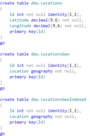
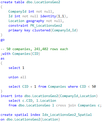
SQL Server database is a collection of the objects that allow us to store and manipulate the data. In theory, SQL Server supports 32,767 databases per instance although the typical installation usually has just several databases. Obviously, the number of the databases SQL Server can handle depends on the load and hardware. It is not unusual to see the servers hosting dozens or even hundreds of small databases.
Every database consists of one or more transaction log and one or more data files. Transaction log stores the information about database transactions and all data modifications made by each session. Every time the data has been modified, SQL Server stores enough information in the transaction log to undo (rollback) or redo (replay) the action.
Every database has one primary data file, which, by default, has .mdf extension. In addition, every database can have secondary database files. Those files, by default, have .ndf extension.
All database files are grouped into the filegroups. Filegroup is the logical unit, which simplifies database administration. They allow the separation between logical object placement and physical database files. When you create the database objects-tables, for example-you specify in what filegroup they should be placed without worrying about underlying data files configuration.
The script shown below creates the database with name OrderEntryDb. That database consists of three filegroups. The primary filegroup has one data file stored on M: drive. Second filegroup- Entities– has one data file on N: drive. Last filegroup- Orders– has two data files stored on O: and P: drives. Finally, there is the transaction log file on L: drive.
create database [OrderEntryDb] on
primary
(name = N'OrderEntryDb', filename = N'm:\OEDb.mdf'),
filegroup [Entities]
(name = N'OrderEntry_Entities_F1', filename = N'n:\OEEntities_F1.ndf'),
filegroup [Orders]
(name = N'OrderEntry_Orders_F1', filename = N'o:\OEOrders_F1.ndf'),
(name = N'OrderEntry_Orders_F2', filename = N'p:\OEOrders_F2.ndf')
log on
(name = N'OrderEntryDb_log', filename = N'l:\OrderEntryDb_log.ldf')
You can see the physical layout of the database and data files below. There are five disks with four data- and one transaction- log files. Dashed rectangles represent the filegroups.
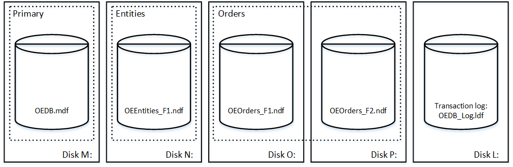
01. Files and Filegroups
Ability to put multiple data files inside the filegroup allows us to spread the load across different storage devices, which would help to improve I/O performance of the system. Transaction log, on the other hand, does not benefit from the multiple files. SQL Server works with transaction log in sequential matter and multple log files just stay idle.
Let’s create a few tables in the database we created. The tables Clients and Articles are placed into Entities filegroup. The table Orders resides in Orders filegroup.
create table dbo.Customers
(
    -- Table columns
) on [Entities];

create table dbo.Articles
(
    -- Table columns
) on [Entities];

create table dbo.Orders
(
    -- Table columns
) on [Orders];
The physical layout of the tables in the database and disks is shown below.
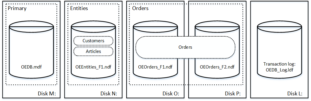
02. Tables and Filegroups
The separation between logical object placement in the filegroups and physical database files allow us to fine-tune the database file layout getting the most from the storage subsystem. For example, independent software vendors (ISV), who are deploying their products to different customers, can adjust the number of database files based on underlying I/O configuration and expected amount of the data during deployment stage. Those changes would be transparent to the developers, who are placing the database objects to the filegroups rather than database files.
It is generally recommended to avoid using PRIMARY filegroup for anything but system objects. Creating separate filegroup or set of the filegroups for the user objects simplifies database administration and disaster recovery especially in case of the large databases.
You can specify initial file size and auto-growth parameters at time when you create the database or add new files to existing database. SQL Server uses proportional fill algorithm when choosing in what data file it should write data to. It writes an amount of data proportionally to the free space available in the files – more free space are in the file, more writes it would handle.
I would recommend that all files in the single filegroup would have the same initial size and auto-growth parameters with grow size defined in megabytes rather than percent. This would help proportional fill algorithm evenly balance write activities across data files.
Every time SQL Server grows the files, it fills newly allocated space in the files with zeros. That process blocks all sessions that need to write to the corresponding file or, in case of transaction log growth, generate transaction log records.
SQL Server always zeroing out transaction log and that behavior cannot be changed. Although, you can control if data files are zeroing out or not by enabling or disabling Instant File Initialization. Enabling Instant File Initialization helps to speed up data file growth and reduces the time required to create or restore the database.
There is the small security risk associated with Instant File Initialization. When this option is enabled, unallocated part of the data file can contain the information from the previously deleted OS files. Database administrators will be able to examine such data.
You can enable Instant File Initialization by adding SA_MANAGE_VOLUME_NAME permission also known as “Perform Volume Maintenance Task” to SQL Server startup account. This can be done under Local Security Policy management application (secpol.msc) as shown below. You need to open properties for “Perform volume maintenance task” permission and add SQL Server startup account to the list of users there.
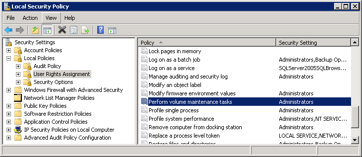
03. Instant File Initialization: Local Security Policy
SQL Server checks if it has Instant File Initialization enabled on startup. You need to restart SQL Server service after you add corresponding permission.
In order to check if permission is enabled, you can use the code from the listing below. This code sets two trace flags that forces SQL Server to put additional information to the error log, creates the small database and reads the content of the log.
-- add more output to error log
dbcc traceon(3004,3605,-1)
go
create database Dummy
go
exec sp_readerrorlog
go
drop database Dummy
go
dbcc traceoff(3004,3605,-1)
go
In case, if Instant File Initialization is not enabled, SQL Server error log shows that SQL Server zeroing mdf data file in addition to zeroing log .ldf file as shown below. When Instant File Initialization is enabled, it would only mention zeroing of the log .ldf file.
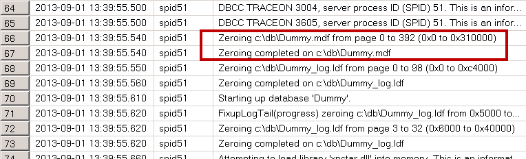
04. Instant File Initialization: Checking if instant file initialization is enabled
Another important database option that controls the database file sizes is Auto Shrink. When this option is enabled, SQL Server regularly shrinks the database files, reduces their size and release space to operating system. This operation is very resource intensive and rarely useful – the database files grow up again after some time when new data comes to the system. Auto Shrink must never be enabled on the database. Moreover, Microsoft would remove that option in the future versions of the SQL Server.