In about a months ago we found that SQL Server does not use non-clustered non-covered indexes in the case, if it expects that it will need to perform the key lookup for more than a few percent of the total table rows. The cost of key lookup is really high, this is random IO operations so it’s cheaper to use the clustered index or table scan instead. The main question is how SQL Server estimates how many rows would be returned. Obviously if you have unique index and equal predicate, the answer is simple. But what about the other cases?

In order to be able to do the estimation, SQL Server maintains the statistics on the indexes and database columns. Good and up to date statistics allow Query Optimizer to assess the cost of the various execution plans and choose the least expensive one.

Let’s take a look at the statistics in more details. First, let’s create a table, populate it with some data and create the index on this table. As you can see the index has the values evenly distributed between 0 and 999.

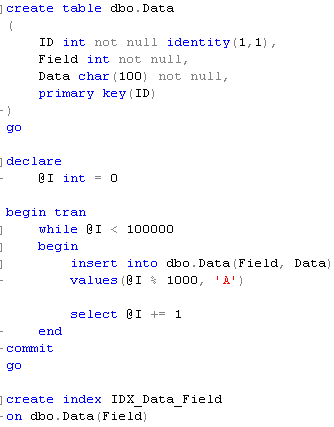
Second, let’s refresh the statistics (we technically don’t need to do that) and call the dbcc_showstatistics stored procedure.

This procedure returns 3 result sets.

Let’s take a look at the first one:

This result set contains the main information. It includes:

1. When statistics was updated
2. How many rows are in the index
3. How many rows have been sampled during statistics creation
4. What is the average key length
5. Is this the string index?
6. Is this the filtered index (in SQL 2008 only).

The 2 most important columns are: what is the time of the last statistics update and how many columns were sampled. The first one shows how up-to-date is the statistics and the second one how full or accurate is the statistics. The last one is interesting. On one hand we don’t want to scan entire (large) table/index for the statistics creation. On other hand we would like to have an accurate statistics. So if data is distributed evenly, the partial scan would work just fine. In other cases it could introduce performance issues during uneven data distribution. One of the examples of such case is the hosting solution where one huge table stored the data for the multiple customers/accounts. Small account obviously has less data than large account. So plan that could be effective in one case could introduce the issues in another.

Let’s look at the second result set.

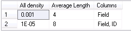
This result set shows the density (1.0 / # of unique values) and the length for the combination of the keys in the composite indexes. Don’t forget that technically every non-clustered index is the composite one – the leaf row (and non-leaf rows for non-unique indexes) includes clustered key values.

The last result set is the most interesting one. It calls the histogram and shows the actual distribution of the data. As the side note – only leftmost column values are included there.

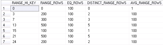
So what does it mean?

1. Range_Hi_Key – this is the upper-bound value for a step
2. Range_Rows – Estimated number of rows in the step with Value < Range_Hi_Key. On other word – number of rows with value > Previus_Range_Hi_Key and < Range_High_Key
3. EQ_Row – Estimated number of rows with value = Range_Hi_Key
4. Distinct_Range_Rows – Estimated # of distinct rows
5. Avg_Range_Rows – Estimated # of rows with duplicate values

Now let’s see what happens if we run the select:

Let’s see what SQL Server does in such case. The set of the values are within the step with Range_Hi_Key = 13.

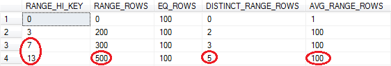
There are 500 rows in the step, 5 distinct values and 100 rows per value. Assuming that data is distributed evenly, SQL Server estimates 400 rows to be returned. That matches the actual number of the rows.

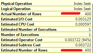
So comparison between Estimated # of Rows and Actual # of rows is one of the first things need to be done during troubleshooting of inefficient plans. It’s completely OK if values are slightly off – for example estimated # = 400 and actual # = 1000, although if the difference is really big most likely there are some problems with the statistics.

The code can be downloaded from here