As we already discussed, implementing of sliding window scenario is one of the biggest benefits you can get from table partitioning. Technically this is quite simple process – when time comes, you have to do 2 different actions:

1. Create the new partition for the future data
2. Switch the oldest partition to the temporary table. After that you can either truncate or archive that data. Possibly even switch this temporary table as the new partition in the historical table.

There are quite a few resources that can show how you can achieve that from the technical standpoint. You can see the example in technet. I’m not going to focus on the implementation details and rather talk about a few less obvious aspects of the implementation.

Usually, we are implementing partitions on the Date basis. We want to purge data daily, monthly or yearly. The problem with this approach is that partition column needs to be included to the clustered index (and as result every non-clustered index). It means extra 4-8 bytes per row from the storage prospective and less efficient index because of bigger row size -> more data pages -> more IO. Obviously there are some cases when nothing can be done and you have to live with it. Although, in a lot of cases, those transaction tables have autoincremented column as part of the row and CI already. In such case, there is the great chance that date column (partition column candidate) would increment the same way with autoincremented ID column. If this is the case, you can think about partitioning by ID instead. This introduces a little bit more work – most likely you’ll
need to maintain another table with (Date,ID) correlations although it would pay itself off because of less storage and better performance requirements. Of course, such assumption cannot guarantee that row always ends up on the right partition. If, for example, insert is delayed, ID could be generated after the split. But in most part of the cases you can live with it.

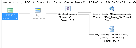
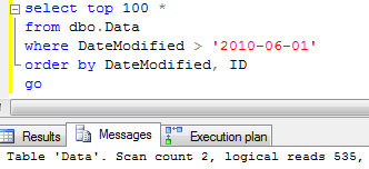
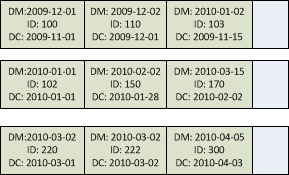
Second thing is creating the new partition. Let’s take a look at the example. First, let’s create the partitioned table and populate it with some data.

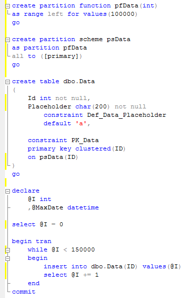
This table has 2 partitions – left with ID <= 100,000 and right, with ID > 100,000. Let’s assume we want to create another partition for the future data (let’s even use ID=200,000 as the split point).

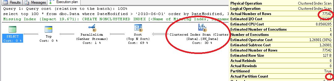
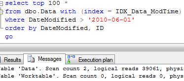
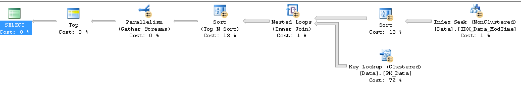
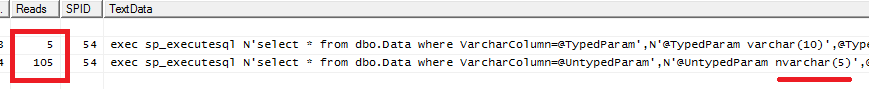
At this point, SQL needs to find out if some data needs to be moved to the new partition. As you can see, it produces a lot of reads. Now let’s try to create another partition with 300,000 as the split point.

As you can see – no IO in such case. So the rule is to always have one additional empty partition reserved. If you decide to accomplish partitioning by ID like we already discussed, make sure:

1. You reserved enough space on the second right-most partition for the time period
2. If ID is identity, insert the dummy row with identity insert on after split in order to start placing the new data to the new partition. Obviously you’ll have holes in the sequence.

Last thing I’d like to mention is locking. Partition switch is metadata operation. Although it will require SCHEMA MODIFICATION (Sch-M) lock. This lock is not compatible with schema stability (SCH-S) lock SQL Server issues during query compilation/execution. If you have OLTP system with a lot of concurrent activity, make sure the code around partition switch/split handles lock timeouts correctly.

Source code is available here

Also – check this post – it could give you some tips how to decrease the possibility of deadlocks during partition/metadata operations.

Last week we started to discuss table partitioning and specified a few cases when partition is really useful. Today I want to focus on the downsides of the process.

First, column used in the partition function needs to be included into the clustered index (and as result all non-clustered indexes). Unless this column is ALREADY part of the clustered index, it means you’re increasing non-clustered index row size. And think about it – you typically partition the large table with millions of rows (what is the reason to partition the small tables?). With such number of rows, index size matters. From both – storage size prospective and index performance.

Another interesting thing – that unless you have rare case when you don’t want index to be aligned, partitioned column should be included into the index definition. It would not increase the row size (CI values are part of the NCI rows anyway), but it could break the indexes you’re using to check uniqueness of the data.

Next, you cannot do partition switch if table is replicated with SQL Server 2005. Fortunately SQL Server 2008 addresses this issue.

Next, you cannot do partition switch if table is referenced by other tables. Typically it’s not an issue for the large transaction tables but still – it could happen.

And now let’s see the worst one. When index is aligned, the data is distributed across multiple partitions. And regular TOP operator does not work anymore. Let’s see that in example. First let’s create the table and populate it with some data.

Now, let’s run the select that get TOP 100 rows:

As you can see the plan is straight-forward – TOP and INDEX SEEK.

Now let’s partition that table by DateCreated.

And run the same select.

Surprisingly it uses clustered index scan. Let’s try to force SQL to use index:

As you can see, it introduces 100 times more reads. Let’s think about it for a minute. Why does it happen?

Think about first example with non-partitioned table. Index data is sorted by DateModified and ID.

So when you run the select like above, SQL Server needs to locate the first row in the index and continue to scan index forward for the next 100 rows. Sweet and simple.

Now let’s think about partition case. We partition index by DateCreated – 3rd column in the index. This column affects the placement of the index row to specific partition. And index is sorted by DateModified and ID only within the partition. See example below – you can see that the row with DateModified = 2010-01-02 can be placed on the first partition because it controlled by DateCreated.

Now let’s think how SQL Server runs the select if it uses the index. For each partition on the table it selects the first row that matches the predicates and scan forward entire partition up to the end. Next, it merges results from all partitions, does the sort and next selects TOP N rows from all the partitions. As you can see, it introduces huge performance hit. I wish SQL Server would be smart enough to scan only N row from each partition, but unfortunately it’s not the case. It scans everything.

Unfortunately there is no simple workaround. This is something you need to live with.

Update (2011-12-18) – Well, there is the workaround that would work in some cases. Check it out here: http://aboutsqlserver.com/2011/12/18/sunday-t-sql-tip-select-top-n-using-aligned-non-clustered-index-on-partitioned-table/

Update (2012-03-11) – Another, more clean and generic workaround – http://aboutsqlserver.com/2012/03/11/sunday-t-sql-tip-aligned-non-clustered-indexes-on-partitioned-table-again/

Source code is available for download.

Next week we will talk about sliding window implementation.

If you’re the lucky user of SQL Server 2005/2008 Enterprise Edition, there is the good chance that you already have table partitioning implemented. Granted, this is one of the best new features introduced in SQL Server 2005 and there were a lot of talks when it was released. Same time, it introduces a few issues and limitations you need to be aware of before the implementation.

I’d like to talk about it in more details. There will be 4 parts in that talk. Today I’m going to be positive – or tell about a few examples when the partitioning benefits you. Next time I’ll show when partitioning is not the best candidate and demonstrate a few interesting side effects you can have in the system. Next, I’ll talk about specific implementation case – Sliding Window and show a couple tricks that can make it more efficient. And at last, I’ll focus on a few other techniques that can replace partitioning if you’re using other editions of SQL Server.

I’d like to talk about it in more details. There will be 4 parts in that talk. Today I’m going to be positive – or tell about a few examples when the partitioning benefits you. Next time I’ll show when partitioning is not the best candidate and demonstrate a few interesting side effects you can have in the system. Next, I’ll talk about specific implementation case – Sliding Window and show a couple tricks that can make it more efficient. And at last, I’ll focus on a few other techniques that can replace partitioning if you’re using other editions of SQL Server.

So what is the table partitioning? There are ton of documentations and white papers (http://msdn.microsoft.com/en-us/library/ms345146%28SQL.90%29.aspx) that can give you a lot of details on implementation level. But let’s keep it simple. Partitioning is the internal storage separation for the subset of the data in the entity. Think about it as about one “virtual” table and multiple “internal” tables which store and combine data seamlessly to the client. Again, I’m not going to focus on implementation and internal details – let’s think about it from the logical standpoint.

Let’s think about specific functional use-cases when it’s beneficial.

1. Sliding window scenario. Assuming you have production database and you need to keep one year worth of the data in the table. Every 1st day of the month you want to purge the data that is more than 1 year old. Without partitioning, you’ll have to use delete statement that would be time consuming and introduce extensive locking in the database (There are a couple ways to avoid it though). With partitioning, you simply switch oldest partition to the temporary table and truncate it. This is metadata operation that takes milliseconds. We will talk about it in more details later
2. Production/historical tables pattern. Think about the previous example when you need to move data to historical table in the same database. Similar approach – you technically move the partition from production to historical tables.
3. Bulk data load. Sometimes it can work in the opposite direction. The data can be loaded to the temporary table and next, that table becomes the new partition. This minimizes the locking during the load. This one has the limited usage though – when system rarely loads the data. You don’t want to do it on daily basis and have hundreds of partitions

The biggest point though is manageability. Different partitions can reside on the different filegroups. It means, you can:

1. Put old, rarely accessed data to the slower drives.
2. Make historical filegroups read-only (helps with backup strategy and improve the performance because SQL Server does not need to obtain locks).
3. Do piecemeal restore and so on.
4. Do index maintenance operations on partition level. You cannot do online index rebuild though

Performance though is the interesting question. SQL Server (especially 2008) has improved algorithms for the parallel execution on partitioned tables. This is definitely good thing for reporting/data warehouse type systems. As for OLTP – it should not be the case. If OLTP system constantly accesses the data from the multiple partitions in one statement, most likely there are some issues in the system. Same time, there are some performance implications I’ll show you next time.

So partitioning is good when you need partitioning. Otherwise it makes the situation worse. Will talk about some performance implications next time.